Integral of Sin(x): Geometric Intuition

You're minding your own business when some punk asks what the integral of $\sin(x)$ means. Your options:

  • Pretend to be asleep (except not in the engineering library again)
  • Canned response: "As with any function, the integral of sine is the area under its curve."
  • Geometric intuition: "The integral of sine is the horizontal distance along a circular path."

Option 1 is tempting, but let's take a look at the others.

Why "Area Under the Curve" is Unsatisfying

Describing an integral as "area under the curve" is like describing a book as a list of words. Technically correct, but misses the message and I suspect you haven't done the assigned reading.

Unless you're trapped in LegoLand, integrals mean something besides rectangles.

Decoding the Integral

My calculus conundrum was not having an intuition for all the mechanics.

When we see:

$\int \sin(x) dx$

We can call on a few insights:

  • The integral is just fancy multiplication. Multiplication accumulates numbers that don't change (3 + 3 + 3 + 3). Integrals add up numbers that might change, based on a pattern (1 + 2 + 3 + 4). But if we squint our eyes and pretend items are identical we have a multiplication.

  • $\sin(x)$ just a percentage. Yes, it's also fancy curve with nice properties. But at any point (like 45 degrees), it's a single percentage from -100% to +100%. Just regular numbers.

  • $dx$ is a tiny, infinitesimal part of the path we're taking. 0 to $x$ is the full path, so $dx$ is (intuitively) a nanometer wide.

Ok. With those 3 intuitions, our rough (rough!) conversion to Plain English is:

The integral of sin(x) multiplies our intended path length (from 0 to x) by a percentage

We intend to travel a simple path from 0 to x, but we end up with a smaller percentage instead. (Why? Because $\sin(x)$ is usually less than 100%). So we'd expect something like 0.75x.

In fact, if $\sin(x)$ did have a fixed value of 0.75, our integral would be:

$\int \text{fixedsin}(x) \ dx = \int 0.75 \ dx = 0.75 \int dx = 0.75x$

But the real $\sin(x)$, that rascal, changes as we go. Let's see what fraction of our path we really get.

Visualize The Change in Sin(x)

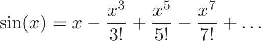
Now let's visualize $\sin(x)$ and its changes:

Here's the decoder key:

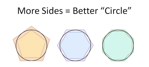
  • $x$ is our current angle in radians. On the unit circle (radius=1), the angle is the distance along the circumference.

  • $dx$ is a tiny change in our angle, which becomes the same change along the circumference (moving 0.01 units in our angle moves 0.01 along the circumference).

  • At our tiny scale, a circle is a a polygon with many sides, so we're moving along a line segment of length $dx$. This puts us at a new position.

With me? With trigonometry, we can find the exact change in height/width as we slide along the circle by $dx$.

By similar triangles, our change just just our original triangle, rotated and scaled.

  • Original triangle (hypotenuse = 1): height = $\sin(x)$, width = $\cos(x)$
  • Change triangle (hypotenuse = dx): height = $\sin(x) dx$, width = $\cos(x) dx$

Now, remember that sine and cosine are functions that return percentages. (A number like 0.75 doesn't have its orientation. It shows up and makes things 75% of their size in whatever direction they're facing.)

So, given how we've drawn our Triangle of Change, $\sin(x) dx$ is our horizontal change. Our plain-English intuition is:

The integral of sin(x) adds up the horizontal change along our path

Visualize The Integral Intuition

Ok. Let's graph this bad boy to see what's happening. With our "$\sin(x) dx$ = tiny horizontal change" insight we have:

As we circle around, we have a bunch of $dx$ line segments (in red). When sine is small (around x=0) we barely get any horizontal motion. As sine gets larger (top of circle), we are moving up to 100% horizontally.

Ultimately, the various $\sin(x) dx$ segments move us horizontally from one side of the circle to the other.

A more technical description:

$\int_0^x \sin(x) dx = \text{horizontal distance traveled on arc from 0 to x}$

Aha! That's the meaning. Let's eyeball it. When moving from $x=0$ to $x=\pi$ we move exactly 2 units horizontally. It makes complete sense in the diagram.

The Official Calculation

Using the Official Calculus Fact that $\int \sin(x) dx = -\cos(x)$ we would calculate:

$ \int_0^\pi \sin(x) dx = -\cos(x) \Big|_0^\pi = -\cos(\pi) - -\cos(0) = -(-1) -(-1) = 1 + 1 = 2$

Yowza. See how awkward it is, those double negations? Why was the visual intuition so much simpler?

Our path along the circle ($x=0$ to $x=\pi$) moves from right-to-left. But the x-axis goes positive from left-to-right. When convert distance along our path into Standard Area™, we have to flip our axes:

Our excitement to put things in the official format stamped out the intuition of what was happening.

Fundamental Theorem of Calculus

We don't really talk about the Fundamental Theorem of Calculus anymore. (Is it something I did?)

Instead of adding up all the tiny segments, just do: end point - start point.

The intuition was staring us in the face: $\cos(x)$ is the anti-derivative, and tracks the horizontal position, so we're just taking a difference between horizontal positions! (With awkward negatives to swap the axes.)

That's the power of the Fundamental Theorem of Calculus. Skip the intermediate steps and just subtract endpoints.

Onward and Upward

Why did I write this? Because I couldn't instantly figure out:

$ \int_0^\pi \sin(x) dx = 2$

This isn't an exotic function with strange parameters. It's like asking someone to figure out $2^3$ without a calculator. If you claim to understand exponents, it should be possible, right?

Now, we can't always visualize things. But for the most common functions we owe ourselves a visual intuition. I certainly can't eyeball the 2 units of area from 0 to $\pi$ under a sine curve.

Happy math.

Appendix: Average Efficiency

As a fun fact, the "average" efficiency of motion around the top of a circle (0 to $\pi$) is: $ \frac{2}{\pi} = .6366 $

So on average, 63.66% of your path's length is converted to horizontal motion.

Appendix: Height controls width?

It seems weird that height controls the width, and vice-versa, right?

If height controlled height, we'd have runaway exponential growth. But a circle needs to regulate itself.

$e^x$ is the kid who eats candy, grows bigger, and can therefore eat more candy.

$\sin(x) $ is the kid who eats candy, gets sick, waits for an appetite, and eats more candy.

Appendix: Area isn't literal

The "area" in our integral isn't literal area, it's a percentage of our length. We visualized the multiplication as a 2d rectangle in our generic integral, but it can be confusing. If you earn money and are taxed, do you visualize 2d area (income * (1 - tax))? Or just a quantity helplessly shrinking?

Area primarily indicates a multiplication happened. Don't let team Integrals Are Literal Area win every battle!

Join 450k Monthly Readers

Enjoy the article? There's plenty more to help you build a lasting, intuitive understanding of math. Join the newsletter for bonus content and the latest updates.

Intuition for Taylor Series (DNA Analogy)

Your body has a strange property: you can learn information about the entire organism from a single cell. Pick a cell, dive into the nucleus, and extract the DNA. You can now regrow the entire creature from that tiny sample.

There's a math analogy here. Take a function, pick a specific point, and dive in. You can pull out enough data from a single point to rebuild the entire function. Whoa. It's like remaking a movie from a single frame.

The Taylor Series discovers the "math DNA" behind a function and lets us rebuild it from a single data point. Let's see how it works.

Pulling information from a point

Given a function like $f(x) = x^2$, what can we discover at a single location?

Normally we'd expect to calculate a single value, like $f(4) = 16$. But there's much more beneath the surface:

  • $f(x)$ = Value of function at point $x$
  • $f'(x)$ = First derivative, or how fast the function is changing (the velocity)
  • $f''(x)$ = Second derivative, or how fast the changes are changing (the acceleration)
  • $f'''(x)$ = Third derivative, or how fast the changes in the changes are changing (acceleration of the acceleration)
  • And so on

Investigating a single point reveals multiple, possibly infinite, bits of information about the behavior. (Some functions have an endless amount of data (derivatives) at a single point).

So, given all this information, what should we do? Regrow the organism from a single cell, of course! (Maniacal cackle here.)

Growing a Function from a point

Our plan is to grow a function from a single starting point. But how can we describe any function in a generic way?

The big aha moment: imagine any function, at its core, is a polynomial (with possibly infinite terms):

\displaystyle{f(x) = c_0 + c_1 x + c_2 x^2 + c_3x^3 + \cdots}

To rebuild our function, we start at a fixed point ($c_0$) and add in a bunch of other terms based on the value we feed it (like $c_1x$). The "DNA" is the values $c_0, c_1, c_2, c_3$ that describe our function exactly.

Ok, we have a generic "function format". But how do we find the coefficients for a specific function like sin(x) (height of angle x on the unit circle)? How do we pull out its DNA?

Time for the magic of 0.

Let's start by plugging in the function value at $x=0$. Doing this, we get:

\displaystyle{f(0) = c_0 + 0 + 0 + 0 + \cdots = c_0}

Every term vanishes except $c_0$, which makes sense: the starting point of our blueprint should be $f(0)$. For $f(x) = \sin(x)$, we can work out $c_0 = \sin(0) = 0$. We have our first bit of DNA!

Getting More DNA

Now that we know $c_0$, how do we isolate $c_1$ in this equation?

\displaystyle{f(x) = c_0 + c_1 x + c_2 x^2 + c_3x^3 + \cdots}

Hrm. A few ideas:

  • Can we set $x = 1$? That gives $f(1) = c_0 + c_1(1) + c_2(1^2) + c_3(1^3) + \cdots$ . Although we know $c_0$, the other constants are summed together. We can't pull out $c_1$ by itself.

  • What if we divide by $x$? This gives:

\displaystyle{\frac{f(x)}{x} = \frac{c_0}{x} + c_1 + c_2 x + c_3x^2 + \cdots}

Then we can set $x=0$ to make the other terms disappear... right? It's a nice idea, except we're now dividing by zero.

Hrm. This approach is really close. How can we almost divide by zero? Using the derivative!

If we take the derivative of the blueprint of $f(x)$, we get:

\displaystyle{f'(x) = (c_0)' + (c_1 x)' + (c_2 x^2)' + (c_3x^3)' + \cdots}

\displaystyle{f'(x) = 0 + c_1 + (2\cdot c_2 x) + (3\cdot c_3x^2) + \cdots}

Every power gets reduced by 1 and the $c_0$, a constant value, becomes zero. It's almost too convenient.

Now we can isolate $c_1$ using our $x=0$ trick:

\displaystyle{f'(0) = 0 + c_1 + (0) + (0) + \cdots = c_1}

In our example, $\sin'(x) = \cos(x)$ so we compute: $f'(0) = \sin'(0) = \cos(0) = 1 = c_1$

Yay, one more bit of DNA! This is the magic of the Taylor series: by repeatedly applying the derivative and setting $x = 0$, we can pull out the polynomial DNA.

Let's try another round:

\displaystyle{f''(x) = 0 + 0 + (2\cdot c_2) + (3\cdot 2 c_3x^1) + \cdots}

After taking the second derivative, the powers are reduced again. The first two terms ($c_0$ and $c_1x$) disappear, and we can again isolate $c_2$ by setting $x=0$:

\displaystyle{f''(0) = 0 + 0 + 2\cdot c_2 + 0 + \cdots}

For our sine example, $\sin'' = -\sin$, so:

\displaystyle{f''(0) = \sin''(0) = -\sin(0) = 0 = 2\cdot c_2}

or $c_2 = 0$.

As we keep taking derivatives, we're performing more multiplications and growing a factorial in front of each term (1!, 2!, 3!).

The Taylor Series for a function around point x=0 is:

\displaystyle{f(x) = f(0) + f'(0) x + \frac{f''(0)}{2!}x^2 + \frac{f'''(0)}{3!}x^3 + \cdots}

(Formally, the Taylor series around the point $x=0$ is called the MacLaurin series.)

The generalized Taylor series, extracted from any point a is:

\displaystyle{f(x) = f(a)+{\frac {f'(a)}{1!}}(x-a)+{\frac {f''(a)}{2!}}(x-a)^{2}+{\frac {f'''(a)}{3!}}(x-a)^{3}+\cdots }

The idea is the same. Instead of our regular blueprint, we use:

\displaystyle{f(x) = c_0 + c_1 (x - a) + c_2 (x-a)^2 + c_3(x-a)^3 + \cdots}

Since we're growing from $f(a)$, we can see that $f(a) = c_0 + 0 + 0 + \dots = c_0$. The other coefficients can be extracted by taking derivatives and setting $x = a$ (instead of $x =0$).

Example: Taylor Series of sin(x)

Plugging in derivatives into the formula above, here's the Taylor series of $\sin(x)$ around $x = 0$:

\displaystyle{\sin(x) = x - \frac{x^3}{3!} + \frac{x^5}{5!} - \frac{x^7}{7!} + \dots}

And here's what that looks like:

A few notes:

1) Sine has infinite terms

Sine is an infinite wave, and as you can guess, needs an infinite number of terms to keep it going. Simpler functions (like $f(x) = x^2 + 3$) are already in their "polynomial format" and don't have infinite derivatives to keep the DNA going.

2) Sine is missing every other term

If we repeatedly take the derivative of sine at x = 0 we get:

\displaystyle{\sin(0) \xrightarrow{\text{derive}} \cos(0) \xrightarrow{\text{derive}} -\sin(0) \xrightarrow{\text{derive}} -\cos(0) \xrightarrow{\text{derive}} \sin(0) \dots}

with values:

\displaystyle{0, 1, 0, -1, \dots}

Ignoring the division by the factorial, we get the pattern:

\displaystyle{(0) + (1)x^1 + (0)x^2 + (-1)x^3 + (0)x^4 + (-1)x^5+ \dots }

So the DNA of sine is something like [0, 1, 0, -1] repeating.

3) Different starting positions have different DNA

For fun, here's the Taylor series of $\sin(x)$ starting at $x =\pi$ (link):

taylor series sin x at x=pi - Wolfram|Alpha 2019-01-18 16-45-04

A few notes:

  • The DNA is now something like [0, -1, 0, 1]. The cycle is similar, but the starting value has changed since we're starting at $x=\pi$.

  • Written as calculated numbers, the denominators 1, 6, 120, 5040 look strange. But they're just every other factorial: 1! = 1, 3! = 6, 5! =120, 7! = 5040. In general, the Taylor series can have gnarly denominators.

  • The $O(x^{12})$ term means there are other components of order (power) $x^{12}$ and higher. Because $\sin(x)$ has infinite derivatives, we have infinite terms and the computer has to cut us off somewhere. (You've had enough Tayloring for today, buddy.)

Application: Function Approximations

A popular use of Taylor series is getting a quick approximation for a function. If you want a tadpole, do you need the DNA for the entire frog?

The Taylor series has a bunch of terms, typically ordered by importance:

\displaystyle{f(x) = f(0) + f'(0) x + \frac{f''(0)}{2!}x^2 + \frac{f'''(0)}{3!}x^3 + \cdots}

  • $c_0 = f(0)$, the constant term, is the exact value at the point
  • $c_1 = f'(0)x$, the linear term, tells us what speed to move from our point
  • $c_2= \frac{f''(0)}{2!}x^2 $, the quadratic term, tells us how much to accelerate away from our point
  • and so on

If we only need a prediction for a few instants around our point, the initial position & velocity may be good enough:

\displaystyle{\text{Linear model} = \text{initial point} + \text{velocity effect} = f(0) + f'(0)x}

If we're tracking for longer, then acceleration becomes important:

\displaystyle{\text{Quadratic model} = \text{initial point} + \text{velocity effect} + \text{acceleration effect}} \displaystyle{ = f(0) + f'(0)x + \frac{1}{2}f''(0)x^2}

As we get further from our starting point, we need more terms to keep our prediction accurate. For example, the linear model $\sin(x) = x$ is a good prediction around $x=0$. As we get further out, we need to account for more terms.

Similarly, $e^x \sim 1 + x$ works well for small interest rates: 1% discrete interest is 1.01 after one time period, 1% continuous interest is a tad higher than 1.01. As time goes on, the linear model falls behind because it ignores the compounding effects.

Application: Comparing Functions

What's a common application of DNA? Paternity tests.

If we have a few functions, we can compare their Taylor series to see if they're related.

Here's the expansions of $\sin(x)$, $\cos(x)$, and $e^x$:

\displaystyle{ \sin x = x - \frac{x^3}{3!} + \frac{x^5}{5!} - \dots \xrightarrow{DNA} [0, 1, 0 -1, \dots] }

\displaystyle{ \cos x = 1 - \frac{x^2}{2!} + \frac{x^4}{4!} - \dots \xrightarrow{DNA} [1, 0, -1, 0, \dots] }

\displaystyle{ e^x = 1 + x + \frac{x^2}{2!} + \frac{x^3}{3!} + \dots \xrightarrow{DNA} [1, 1, 1, 1, \dots] }

There's a family resemblence in the sequences, right? Clean powers of $x$ divided by a factorial?

One problem is the sequence for $e^x$ has positive terms, while sine and cosine alternate signs. How can we link these together?

Euler's great insight was realizing an imaginary number could swap the sign from positive to negative:

{\begin{aligned}e^{ix}&=1+ix+{\frac {(ix)^{2}}{2!}}+{\frac {(ix)^{3}}{3!}}+{\frac {(ix)^{4}}{4!}}+{\frac {(ix)^{5}}{5!}}+{\frac {(ix)^{6}}{6!}}+{\frac {(ix)^{7}}{7!}}+{\frac {(ix)^{8}}{8!}}+\cdots \\[8pt]&=1+ix-{\frac {x^{2}}{2!}}-{\frac {ix^{3}}{3!}}+{\frac {x^{4}}{4!}}+{\frac {ix^{5}}{5!}}-{\frac {x^{6}}{6!}}-{\frac {ix^{7}}{7!}}+{\frac {x^{8}}{8!}}+\cdots \\[8pt]&=\left(1-{\frac {x^{2}}{2!}}+{\frac {x^{4}}{4!}}-{\frac {x^{6}}{6!}}+{\frac {x^{8}}{8!}}-\cdots \right)+i\left(x-{\frac {x^{3}}{3!}}+{\frac {x^{5}}{5!}}-{\frac {x^{7}}{7!}}+\cdots \right)\\[8pt]&=\cos x+i\sin x.\end{aligned}}

Whoa. Using an imaginary exponent and separating into odd/even powers reveals that sine and cosine are hiding inside the exponential function. Amazing.

Although this proof of Euler's Formula doesn't show why the imaginary number makes sense, it reveals the baby daddy hiding backstage.

Appendix: Assorted Aha! Moments

Relationship to Fourier Series

The Taylor Series extracts the "polynomial DNA" and the Fourier Series/Transform extracts the "circular DNA" of a function. Both see functions as built from smaller parts (polynomials or exponential paths).

Does the Taylor Series always work?

This gets into mathematical analysis beyond my depth, but certain functions aren't easily (or ever) approximated with polynomials.

Notice that powers like $x^2, x^3$ explode as $x$ grows. In order to have a slow, gradual curve, you need an army of polynomial terms fighting it out, with one winner barely emerging. If you stop the train too early, the approximation explodes again.

For example, here's the Taylor Series for $\ln(1 + x)$. The black line is the curve we want, and adding more terms, even dozens, barely gets us accuracy beyond $x=1.0$. It's just too hard to maintain a gentle slope with terms that want to run hog wild.

source

In this case, we only have a radius of convergence where the approximation stays accurate (such as around $|x| < 1$).

Turning geometric to algebraic definitions

Sine is often defined geometrically: the height of a line on a circular figure.

Turning this into an equation seems really hard. The Taylor Series gives us a process: If we know a single value and how it changes (the derivative), we can reverse-engineer the DNA.

Similarly, the description of $e^x$ as "the function with its derivative equal to the current value" yields the DNA [1, 1, 1, 1], and polynomial $f(x) = 1 + \frac{1}{1!}x + \frac{1}{2!}x^2 + \frac{1}{3!}x^3 + \dots $. We went from a verbal description to an equation.

Phew! A few items to ponder.

Happy math.

Join 450k Monthly Readers

Enjoy the article? There's plenty more to help you build a lasting, intuitive understanding of math. Join the newsletter for bonus content and the latest updates.

How to Add 1 through 100 using Calculus

Earlier we saw a few ways to add a set of numbers (1 to 10).

adding 1 to 100 strategies

And the formula we found was:

\displaystyle{\text{Sum from 1 to n} = \frac{n(n+1)}{2}}

\displaystyle{\text{Sum from 1 to 100} = \frac{100(100+1)}{2} = (50)(101) = 5050}

It seems that regular arithmetic, algebra, geometry, or even statistics could help work out the equation.

But how about Calculus? Is this bringing a nuclear missile to a gun fight?

Let's find out.

The sequence to add (1 2 3 4 5 6 7 8 9 10...) looks a lot like $f(x) = x$. At every position on the x-axis, we put in a number and get the same one out.

Intuitively, the integral is "repeatedly adding a bunch of stuff" -- it seems like we could put it to work. From the rules of Calculus (or using Wolfram Alpha) we get this:

\displaystyle{
\int x = \frac{1}{2} x^2
}

Intuitively: Add up things following the $f(x) = x$ pattern and you end up with $\frac{1}{2} x^2$.

Well, let's see: the actual sum from 1 to 100 is 5050. But using the Calculus equation we get:

\displaystyle{
\frac{1}{2} x^2 = \frac{1}{2}100^2 = \frac{10,000}{2} = 5000
}

Uh oh: there's a difference. What's going on?

Calculus works with continuous patterns, and we used a discrete one.

Here's what's happening:

calculus add area under x

Calculus was built to measure smoothly changing functions, like a line, parabola, circle, etc. The pattern we have is a jumpy staircase (going from 1 to 2 without ever passing through 1.5, or 1.1, or 1.0001). In math class, books harp on analyzing whether a function is "continuous", aka changes smoothly enough for Calculus to work.

So when a pattern changes smoothly, Calculus works great. If a pattern changes suddenly, Calculus can only give an approximate answer. So what's the plan?

Use Calculus where possible, on the smooth part, and adjust for errors in the jumpy part.

calculus integral of x discrete

The area under the line is the integral. We a bunch of triangles above the line we need to include.

  • How many of them? 1 for each item (x)
  • How big are they? They're half a of a 1x1 square, so they have area 1/2.
  • What's the total area to add back in? $x \frac{1}{2} = \frac{x}{2}$

So our final formula should be

\displaystyle{\text{Integral} + \text{Adjustment} = \frac{1}{2} x^2 + \frac{x}{2}}

Aha! Learning Calculus doesn't mean we hunt around for Official Calculus Problems.

Nope. Take your scenario (adding 1 to 100) and realize what Calculus brings to the table: finding patterns in smoothly changing functions. Use Calculus on the smooth parts and adjust (or ignore) the other parts.

(Ironically, Calculus works by making jumpy approximations for smooth functions, and is in fact "jumpy" under the hood. If you are planning on working with jumpy patterns, use Discrete Calculus.)

Example: Adding the first n squares

Let's take this further: what's your guess for the sum of the first 100 square numbers?

\displaystyle{1^2 + 2^2 + 3^2 + 4^2 + ... + 100^2}

Hrm. Getting the exact formula is tricky. But maybe we don't need the exact count, just an estimate.

With Calculus, we'd say: The pattern isn't continuous, but it looks like $f(x) = x^2$. Let's integrate x^2 from 0 to 100.

\displaystyle{
\int x^2 = \frac{1}{3} x^3
}

The indefinite integral is $\frac{1}{3} x^3 $, the running total for how much we have. From 0 to 100 it would be

\displaystyle{
\frac{1}{3}100^3 = \frac{1,000,000}{3} \sim 333,333
}

That's our guess, without a calculator. And the actual answer? 338350.

calculus area under x squared

How close were we? 99.9%. Not bad for something we worked out by hand in a minute!

Truly internalizing Calculus means it helps other elements of your math understanding, even regular addition problems.

Happy math.

PS. To keep building your intuition, check out the Calculus Guide.

Join 450k Monthly Readers

Enjoy the article? There's plenty more to help you build a lasting, intuitive understanding of math. Join the newsletter for bonus content and the latest updates.

Quick Insight: Easier Arithmetic With Calculus

Let's say you had to estimate 1 + 2 + 3 + 4 + 5 + 6 + 7 + ... + 100.

What would you do? Well, you could work out the exact formula:

\displaystyle{\frac{(n + 1)(n)}{2}}

and plug in n=100 to get 5050.

But we just want a rough answer. You have a list of numbers, they follow a simple pattern, and want a quick estimate. What to do?

The "easy" way (well, the Calculus way) is to realize 1 + 2 + 3 + 4 is about the same as $f(x) = x$. The first element is f(1) = 1, the second is f(2) = 2, and so on.

From here, we can take the integral:

\displaystyle{ \int x = \frac{1}{2} x^2 }

We usually see the integral as a formal, elegant operation, which artfully accumulates one function and returns another. Informally, we're squashing everything together in that bad mamma-jamma and seeing how much there is.

The result $\frac{1}{2} x^2$ should be pretty close to what we want.

calculus add area under x

The exact total is our staircase-like pattern, which accumulates to 5050.

The approximate answer is the area of that triangle, $\frac{1}{2} base * height = \frac{1}{2} 100 * 100 = 5000$. The difference is because of the corners in the staircase which overhang. $\frac{x}{2}$ is one-half, x times (the size of overhang (1/2) times the number of pieces (x)).

The net result is using a smooth, easy-to-measure shape to approximate a jagged, tedious-to-measure one. (This is a bit of Calculus inception, since we usually use rectangles to approximate smooth shapes.)

More Estimates

This tactic works for other sequences:

What's the sum of the first 10 square numbers? 1 + 4 + 9 + 16 + 25 + ... + 100 = ?

Hrm. The formula is probably tricky to work out. But without our Calculus-infused Arithmetic, a quick guess would be:

calculus add square numbers x squared

\displaystyle{\int x^2 = \frac{1}{3} x^3}

Our first hunch should be "one third of 10^3" or 333. But as we saw before, there's an "overhang" that we missed. Let's call it 10%, for an estimate of 330 + 10% ~ 370.

The exact answer is 385. Not bad! The actual formula is:

\displaystyle{P_{n}=\sum _{k=1}^{n}k^{2}={\frac {n(n+1)(2n+1)}{6}}={\frac {2n^{3}+3n^{2}+n}{6}}={\frac {n^{3}}{3}}+{\frac {n^{2}}{2}}+{\frac {n}{6}} }

I'd say $\frac{x^3}{3}$ isn't bad for a few seconds of work.

Data doubles every year. What does lifetime usage look like?

The integral (squashed-together total) of an exponential is an exponential. In Calculus terms,

\displaystyle{\int e^x = e^x}

The key insight is that all exponential growth is just a variation of $e^x$. If $e^x$ accumulates exponentially, so will $2^x$.

So the total usage to date will also follow an exponential pattern, doubling every year also. Contrast this with a usage pattern of "1 + 2 + 3 + 4 ..." -- we grow linearly ($f(x) = x$), but total usage accumulates quadratically ($\frac{1}{2}x^2$).

My goal is to incorporate math thinking into everyday scenarios. We start with an arithmetic question, convert it to a geometry puzzle (how big is the staircase?), and then use calculus to approximate it.

I know a concept is clicking when I can switch between a few styles of thought. Imagine the problem as a script: how would Spielberg, Tarantino, or Scorsese direct it? Each field takes a different look. (To learn how to think with Calculus, check out the Calculus Guide.)

Happy math.

Join 450k Monthly Readers

Enjoy the article? There's plenty more to help you build a lasting, intuitive understanding of math. Join the newsletter for bonus content and the latest updates.

Abstraction Practice: Calculus Graphs

Let's practice our abstraction skills by simplifying concepts in Calculus.

Last time, we saw how abstraction simplifies ideas.

math abstraction example lions

After removing enough detail, a photo of lions turns into the notion of quantity (where n happens to be 3 in this case).

Let's apply this to a function like $f(x) = x^2$. What's the simplified essence?

Here were my first thoughts as I worked through the idea:

math abstract change

Abstraction 1: Multiple shapes

First, look at a few representations of $x^2$. The common cliche is that it represents a square of side x, but we can be more creative. What about a rectangle with sides $\frac{1}{2}x$ and $2x$? How about a portion of a circle? (If $\text{area} = \pi r^2$ then $\frac{1}{\pi}$ (32%) should leave us with $r^2$.)

Abstraction 2: Examine the specific changes

Next, look at the changes that happen with each of our shapes. The square gets equal lengths added to each side. The rectangle gets a "long, skinny" and "short, fat" added to each side. (The corners can be ignored for now.)

The changes to the circle are the simplest, with a small arc being added.

Abstraction 3: Make the changes general

Like the lion scenario above, we have a unique representation of each change ("three lion icons"). Let's make the changes generic (three lines) by finding a common format.

Here, we "melt down" each change until it resembles a straight line. Because the square, rectangle, and circle all represent $x^2$, the same line can describe the changes they undergo. Neat!

Now that's some nice abstractin', let's keep it going:

math rate of change directional arrow

Abstraction 4: Separate the line

The orange "change line" is actually a transition between a starting and ending position. If we represent the start and end as blue dots, the height of the line is the amount of change between them.

Notice how we make an angled line as well: the input change (blue line) and output change (orange line) trace out the rate of change (green line).

Abstraction 5: Show every state and angle

Rather than picking specific starting and endpoint positions, graph every position (blue curve) and every rate of change (green line at each point).

The blue curve actually generates the green line: at any point, we can draw the tangent line and see the "change angle" to the next neighbor.

The Number/Angle Abstraction

Here's where I get excited. On a graph, we're used to literal representations: we need a bigger line to represent a bigger change. But an angle (a certain ratio of height:width) represents every number in the same amount of space!

number and angle arrow

  • 0:1 is 0 degrees

  • 1:1 is 45 degrees

  • 2:1 is 63.4 degrees ($\arctan(2) = 63.4$)

  • 100:1 is 89.4 degrees ($\arctan(100) = 89.4$)

By using an angle, we've curled the number line into a format that fits into any space. Even a giant number like 10,000,000,000 can be written with the same effort as "1". Must bigger numbers take up more room?

We have a clean abstraction: The curve shows every possible scenario, and the angle quantifies the rate of change. In a way, the curve "writes down" its rate of change at every point.

Yowza. Maybe we discussed this in class, but I didn't think of it this way until trying to abstract each step.

This was a peek into an organic "aha-finding" technique: start with a specific idea, keep generalizing, and see what insights emerge.

Happy math.

Join 450k Monthly Readers

Enjoy the article? There's plenty more to help you build a lasting, intuitive understanding of math. Join the newsletter for bonus content and the latest updates.

Analogy: The Calculus Camera

Imagine you're a photographer. You come across a beautiful, reflective object: a metal sphere, a calm lake, a mirrored room. Seems like a good photo op, right?

Sure, except your photos come out like this:

(An old-timey selfie. Source.)

The dilemma: You need a camera for the photo, but don't want the camera in the photo. The instrument shouldn't appear inside the subject. (Hubert, you're leaving scalpels in the patient again.)

So, we need an isolated photo of a shiny object. What can we do?

  • Shrink it down: Make the camera as small as possible. Microscopic, a fleck of dust. But even that speck will show up on the sphere. Take the photo, and fix the blemish with our best guess given the surrounding pixels.

  • Go invisible: Make the camera unobservable to the subject: make it from perfectly transparent glass, or actively camouflage with your surroundings (like an octopus). The camera is there, looking at the subject, but the subject cannot notice it.

In Calculus, a function like $f(x) = x^2$ is our subject. Limits (shrinking) and infinitesimals (invisibility) are how we take photos without our reflection getting in the way.

Taking a Photo of a Function

Consider a function like $f(x) = 2x + 3$. If I take a photo with my camera, I get:

  • Before: $f(x) = 2x + 3$
  • After: $f(x + \text{camera}) = 2(x + \text{camera}) + 3 = 2x + 3 + 2\text{camera}$

We have the original function, and put the camera into the scene. The result is the original function ($2x + 3$) and the camera observing "2". That is, the camera thinks "2" is how much the function has changed. (And yes, $\frac{d}{dx} 2x + 3 = 2$.)

Ok. Now take a function like $f(x) = x^2$. Again, let's put the camera into the scene to observe changes:

  • Before: $f(x) = x^2$
  • After: $f(x + \text{camera}) = (x + \text{camera})^2 = x^2 + 2x \cdot \text{camera} + \text{camera}^2$

Hrm. The camera is directly observing some changes ($2x \cdot \text{camera}$) but there's another $\text{camera}^2$ term: the camera is observing its own reflection! The term $\text{camera}^2$ only exists because we have a camera in the first place. It's an illusion.

What's the fix?

  1. List all the changes the camera sees:

    \begin{aligned}
f(x + \text{camera}) - f(x) &= [x^2 + 2x \cdot \text{camera} + \text{camera}^2] - [x^2] \\
&= 2x \cdot \text{camera} + \text{camera}^2
\end{aligned}

  2. Figure out what the camera directly observed. We divide to see what was "attached" to the camera:

    \displaystyle{\frac{2x \cdot \text{camera} + \text{camera}^2}{\text{camera}} = 2x + \text{camera}}

  3. Remove "reflections" where the camera saw itself:

    \displaystyle{2x + \text{camera} \rightarrow 2x}

calculus camera analogy

From a technical perspective, the last step happens by shrinking the camera to zero (limits) or letting the camera be invisible (infinitesimals).

Neat, eh? We're reframing the process of finding the derivative: make a change, see what the direct effects are, remove the artifacts. The concept of "what the camera directly sees" and the camera's "reflection" help settle my mind about throwing away terms that appear to be there.

In math, we have fancy terms like linear and non-linear functions. We can think in terms of "shiny" or "dull" functions.

Linear functions are dull because they only have terms like $x$ or constant values -- the camera can attach directly, and there's no reflection. Non-linear functions have self-interactions (like $x^2$) which means the camera has a chance to see itself. Reflections need to be removed.

With multiple subjects [$f(x)$, $g(x)$] or multiple cameras (for the x, y and z axis) we get cross terms like $df \cdot dg$ or $dx \cdot dy$. The goal is the same: remove unnecessary self- and cross-reflections from the final result. Show what the camera directly sees.

A few related blog posts on limits:

The role of dx

Regular calculus books use $dx$ as the camera to detect change. The goal is to introduce a change ($dx$), then get the difference ($f(x + dx) - f(x)$).

This difference (for example, $2x \cdot dx + dx^2$) isolates the changes that $dx$ is directly responsible for ("sees"). We can then divide by $dx$ to get the change as a rate (how much we got out for how much we put in).

The concern is the same: the change $dx$ may have reflections ($dx^2$) that need to be removed.

Real-World Application: The Hawthorne Effect

The Hawthorne Effect is where people behave differently when being studied. The study itself is appearing in the results.

If you ask people to enter a study about their eating, exercise, reading, or sleeping habits, those behaviors will change. (Gotta look good for the camera! Where are those Greek philosophers I'd always meant to read?)

Math gives us a few suggestions:

  • Shrink the effect: Make the study as non-intrusive as possible (like an iPhone passively monitoring your steps). Even then, figure out how much the results are skewed and adjust for this. (You left your phone on the washing machine again, you sly dog.)

  • Make the observations invisible: Imagine you don't know when the study is going to start. "Sometime in the next 20 years we'll silently observe your grocery shopping habits. Sign here." Hrm. You won't change your behavior for 20 years "just in case", so you'll just be you.

Think math only applies to equations? Hah. Only if we don't internalize the underlying concept.

Happy math.

Join 450k Monthly Readers

Enjoy the article? There's plenty more to help you build a lasting, intuitive understanding of math. Join the newsletter for bonus content and the latest updates.

An Intuitive Introduction To Limits

Limits, the Foundations Of Calculus, seem so artificial and weasely: “Let x approach 0, but not get there, yet we’ll act like it’s there… ” Ugh.

Here’s how I learned to enjoy them:

  • What is a limit? Our best prediction of a point we didn’t observe.
  • How do we make a prediction? Zoom into the neighboring points. If our prediction is always in-between neighboring points, no matter how much we zoom, that’s our estimate.
  • Why do we need limits? Math has “black hole” scenarios (dividing by zero, going to infinity), and limits give us an estimate when we can’t compute a result directly.
  • How do we know we’re right? We don’t. Our prediction, the limit, isn’t required to match reality. But for most natural phenomena, it sure seems to.

Limits let us ask “What if?”. If we can directly observe a function at a value (like x=0, or x growing infinitely), we don’t need a prediction. The limit wonders, “If you can see everything except a single value, what do you think is there?”.

When our prediction is consistent and improves the closer we look, we feel confident in it. And if the function behaves smoothly, like most real-world functions do, the limit is where the missing point must be.

Key Analogy: Predicting A Soccer Ball

Pretend you’re watching a soccer game. Unfortunately, the connection is choppy:

soccer limit analogy calculus

Ack! We missed what happened at 4:00. Even so, what’s your prediction for the ball’s position?

Easy. Just grab the neighboring instants (3:59 and 4:01) and predict the ball to be somewhere in-between.

And… it works! Real-world objects don’t teleport; they move through intermediate positions along their path from A to B. Our prediction is “At 4:00, the ball was between its position at 3:59 and 4:01”. Not bad.

With a slow-motion camera, we might even say “At 4:00, the ball was between its positions at 3:59.999 and 4:00.001”.

Our prediction is feeling solid. Can we articulate why?

  • The predictions agree at increasing zoom levels. Imagine the 3:59-4:01 range was 9.9-10.1 meters, but after zooming into 3:59.999-4:00.001, the range widened to 9-12 meters. Uh oh! Zooming should narrow our estimate, not make it worse! Not every zoom level needs to be accurate (imagine seeing the game every 5 minutes), but to feel confident, there must be some threshold where subsequent zooms only strengthen our range estimate.

  • The before-and-after agree. Imagine at 3:59 the ball was at 10 meters, rolling right, and at 4:01 it was at 50 meters, rolling left. What happened? We had a sudden jump (a camera change?) and now we can’t pin down the ball’s position. Which one had the ball at 4:00? This ambiguity shatters our ability to make a confident prediction.

With these requirements in place, we might say “At 4:00, the ball was at 10 meters. This estimate is confirmed by our initial zoom (3:59-4:01, which estimates 9.9 to 10.1 meters) and the following one (3:59.999-4:00.001, which estimates 9.999 to 10.001 meters)”.

Limits are a strategy for making confident predictions.

Exploring The Intuition

Let’s not bring out the math definitions just yet. What things, in the real world, do we want an accurate prediction for but can’t easily measure?

What’s the circumference of a circle?

Finding pi “experimentally” is tough: bust out a string and a ruler?

We can’t measure a shape with seemingly infinite sides, but we can wonder “Is there a predicted value for pi that is always accurate as we keep increasing the sides?”

Archimedes figured out that pi had a range of

\displaystyle{3 \frac{10}{71} < \pi < 3 \frac{1}{7} }

using a process like this:

circle limit approximation

It was the precursor to calculus: he determined that pi was a number that stayed between his ever-shrinking boundaries. Nowadays, we have modern limit definitions of pi.

What does perfectly continuous growth look like?

e, one of my favorite numbers, can be defined like this:

\displaystyle{e = \lim_{n\to\infty} \left( 1 + \frac{1}{n} \right)^n}

continuous growth limit approximation

We can’t easily measure the result of infinitely-compounded growth. But, if we could make a prediction, is there a single rate that is ever-accurate? It seems to be around 2.71828…

Can we use simple shapes to measure complex ones?

Circles and curves are tough to measure, but rectangles are easy. If we could use an infinite number of rectangles to simulate curved area, can we get a result that withstands infinite scrutiny? (Maybe we can find the area of a circle.)

calculus circle to rings

Can we find the speed at an instant?

Speed is funny: it needs a before-and-after measurement (distance traveled / time taken), but can’t we have a speed at individual instants? Hrm.

Limits help answer this conundrum: predict your speed when traveling to a neighboring instant. Then ask the “impossible question”: what’s your predicted speed when the gap to the neighboring instant is zero?

Note: The limit isn’t a magic cure-all. We can’t assume one exists, and there may not be an answer to every question. For example: Is the number of integers even or odd? The quantity is infinite, and neither the “even” nor “odd” prediction stays accurate as we count higher. No well-supported prediction exists.

For pi, e, and the foundations of calculus, smart minds did the proofs to determine that “Yes, our predicted values get more accurate the closer we look.” Now I see why limits are so important: they’re a stamp of approval on our predictions.

The Math: The Formal Definition Of A Limit

Limits are well-supported predictions. Here’s the official definition:

\displaystyle{ \lim_{x \to c}f(x) = L } 
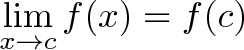
means for all real ε > 0 there exists a real δ > 0 such that for all x with 0 < |x − c| < δ, we have |f(x) − L| < ε

Let’s make this readable:

Math EnglishHuman English
\displaystyle{ \lim_{x \to c}f(x) = L \text{ means } }
When we “strongly predict” that f(c) = L, we mean
for all real ε > 0for any error margin we want (+/- .1 meters)
there exists a real δ > 0there is a zoom level (+/- .1 seconds)
such that for all x with 0 < |x − c| < δ, we have |f(x) − L| < εwhere the prediction stays accurate to within the error margin

There’s a few subtleties here:

  • The zoom level (delta, δ) is the function input, i.e. the time in the video
  • The error margin (epsilon, ε) is the most the function output (the ball’s position) can differ from our prediction throughout the entire zoom level
  • The absolute value condition (0 < |x − c| < δ) means positive and negative offsets must work, and we’re skipping the black hole itself (when |x – c| = 0).

We can’t evaluate the black hole input, but we can say “Except for the missing point, the entire zoom level confirms the prediction $f(c) = L$.” And because $f(c) = L$ holds for any error margin we can find, we feel confident.

Could we have multiple predictions? Imagine we predicted L1 and L2 for f(c). There’s some difference between them (call it .1), therefore there’s some error margin (.01) that would reveal the more accurate one. Every function output in the range can’t be within .01 of both predictions. We either have a single, infinitely-accurate prediction, or we don’t.

Yes, we can get cute and ask for the “left hand limit” (prediction from before the event) and the “right hand limit” (prediction from after the event), but we only have a real limit when they agree.

A function is continuous when it always matches the predicted value (and discontinuous if not):

\displaystyle{\lim_{x \to c}{f(x)} = f(c)}

Calculus typically studies continuous functions, playing the game “We’re making predictions, but only because we know they’ll be correct.”

The Math: Showing The Limit Exists

We have the requirements for a solid prediction. Questions asking you to “Prove the limit exists” ask you to justify your estimate.

For example: Prove the limit at x=2 exists for

\displaystyle{f(x) = \frac{(2x+1)(x-2)}{(x - 2)}}

The first check: do we even need a limit? Unfortunately, we do: just plugging in “x=2” means we have a division by zero. Drats.

But intuitively, we see the same “zero” (x – 2) could be cancelled from the top and bottom. Here’s how to dance this dangerous tango:

  • Assume x is anywhere except 2 (It must be! We’re making a prediction from the outside.)
  • We can then cancel (x – 2) from the top and bottom, since it isn’t zero.
  • We’re left with f(x) = 2x + 1. This function can be used outside the black hole.
  • What does this simpler function predict? That f(2) = 2*2 + 1 = 5.

So f(2) = 5 is our prediction. But did you see the sneakiness? We pretended x wasn’t 2 [to divide out (x-2)], then plugged in 2 after that troublesome item was gone! Think of it this way: we used the simple behavior from outside the event to predict the gnarly behavior at the event.

We can prove these shenanigans give a solid prediction, and that f(2) = 5 is infinitely accurate.

For any accuracy threshold (ε), we need to find the “zoom range” (δ) where we stay within the given accuracy. For example, can we keep the estimate between +/- 1.0?

Sure. We need to find out where

\displaystyle{|f(x) - 5| < 1.0}

so


\begin{aligned}
|2x + 1 - 5| &< 1.0 \\
|2x - 4| &< 1.0 \\
|2(x - 2)| &< 1.0 \\
2|(x - 2)| &< 1.0 \\
|x - 2| &< 0.5
\end{aligned}

In other words, x must stay within 0.5 of 2 to maintain the initial accuracy requirement of 1.0. Indeed, when x is between 1.5 and 2.5, f(x) goes from f(1.5) = 4 to and f(2.5) = 6, staying +/- 1.0 from our predicted value of 5.

We can generalize to any error tolerance (ε) by plugging it in for 1.0 above. We get:

\displaystyle{|x - 2| < 0.5 \cdot \epsilon}

If our zoom level is “δ = 0.5 * ε”, we’ll stay within the original error. If our error is 1.0 we need to zoom to .5; if it’s 0.1, we need to zoom to 0.05.

This simple function was a convenient example. The idea is to start with the initial constraint (|f(x) – L| < ε), plug in f(x) and L, and solve for the distance away from the black-hole point (|x – c| < ?). It’s often an exercise in algebra.

Sometimes you’re asked to simply find the limit (plug in 2 and get f(2) = 5), other times you’re asked to prove a limit exists, i.e. crank through the epsilon-delta algebra.

Flipping Zero and Infinity

Infinity, when used in a limit, means “grows without stopping”. The symbol ∞ is no more a number than the sentence “grows without stopping” or “my supply of underpants is dwindling”. They are concepts, not numbers (for our level of math, Aleph me alone).

When using ∞ in a limit, we’re asking: “As x grows without stopping, can we make a prediction that remains accurate?”. If there is a limit, it means the predicted value is always confirmed, no matter how far out we look.

But, I still don’t like infinity because I can’t see it. But I can see zero. With limits, you can rewrite

\displaystyle{\lim_{x \to \infty}}

as

\displaystyle{\lim_{\frac{1}{x} \to 0}}

You can get sneaky and define y = 1/x, replace items in your formula, and then use

\displaystyle{\lim_{y \to 0^+}}

so it looks like a normal problem again! (Note from Tim in the comments: the limit is coming from the right, since x was going to positive infinity). I prefer this arrangement, because I can see the location we’re narrowing in on (we’re always running out of paper when charting the infinite version).

Why Aren’t Limits Used More Often?

Imagine a kid who figured out that “Putting a zero on the end” made a number 10x larger. Have 5? Write down “5” then “0” or 50. Have 100? Make it 1000. And so on.

He didn’t figure out why multiplication works, why this rule is justified… but, you’ve gotta admit, he sure can multiply by 10. Sure, there are some edge cases (Would 0 become “00”?), but it works pretty well.

The rules of calculus were discovered informally (by modern standards). Newton deduced that “The derivative of $x^3$ is $3x^2$” without rigorous justification. Yet engines whirl and airplanes fly based on his unofficial results.

The calculus pedagogy mistake is creating a roadblock like “You must know Limits™ before appreciating calculus”, when it’s clear the inventors of calculus didn’t. I’d prefer this progression:

  • Calculus asks seemingly impossible questions: When can rectangles measure a curve? Can we detect instantaneous change?
  • Limits give a strategy for answering “impossible” questions (“If you can make a prediction that withstands infinite scrutiny, we’ll say it’s ok.”)
  • They’re a great tag-team: Calculus explores, limits verify. We memorize shortcuts for the results we verified with limits ($\frac{d}{dx} x^3 = 3x^2$), just like we memorize shortcuts for the rules we verified with multiplication (adding a zero means times 10). But it’s still nice to know why the shortcuts are justified.

Limits aren’t the only tool for checking the answers to impossible questions; infinitesimals work too. The key is understanding what we’re trying to predict, then learning the rules of making predictions.

Happy math.

Join 450k Monthly Readers

Enjoy the article? There's plenty more to help you build a lasting, intuitive understanding of math. Join the newsletter for bonus content and the latest updates.

How To Understand Derivatives: The Quotient Rule, Exponents, and Logarithms

Last time we tackled derivatives with a "machine" metaphor. Functions are a machine with an input (x) and output (y) lever. The derivative, dy/dx, is how much "output wiggle" we get when we wiggle the input:

simple function

Now, we can make a bigger machine from smaller ones (h = f + g, h = f * g, etc.). The derivative rules (addition rule, product rule) give us the "overall wiggle" in terms of the parts. The chain rule is special: we can "zoom into" a single derivative and rewrite it in terms of another input (like converting "miles per hour" to "miles per minute" -- we're converting the "time" input).

And with that recap, let's build our intuition for the advanced derivative rules. Onward!

Division (Quotient Rule)

Ah, the quotient rule -- the one nobody remembers. Oh, maybe you memorized it with a song like "Low dee high, high dee low...", but that's not understanding!

It's time to visualize the division rule (who says "quotient" in real life?). The key is to see division as a type of multiplication:

\displaystyle{h = \frac{f}{g} = f \cdot \frac{1}{g}}

derivative product rule

We have a rectangle, we have area, but the sides are "f" and "1/g". Input x changes off on the side (by dx), so f and g change (by df and dg)... but how does 1/g behave?

Chain rule to the rescue! We can wrap up 1/g into a nice, clean variable and then "zoom in" to see that yes, it has a division inside.

So let's pretend 1/g is a separate function, m. Inside function m is a division, but ignore that for a minute. We just want to combine two perspectives:

  • f changes by df, contributing area df * m = df * (1 / g)
  • m changes by dm, contributing area dm * f = ?

We turned m into 1/g easily. Fine. But what is dm (how much 1/g changed) in terms of dg (how much g changed)?

We want the difference between neighboring values of 1/g: 1/g and 1/(g + dg). For example:

  • What's the difference between 1/4 and 1/3? 1/12
  • How about 1/5 and 1/4? 1/20
  • How about 1/6 and 1/5? 1/30

How does this work? We get the common denominator: for 1/3 and 1/4, it's 1/12. And the difference between "neighbors" (like 1/3 and 1/4) will be 1 / common denominator, aka 1 / (x * (x + 1)). See if you can work out why!

\displaystyle{\frac{1}{x + 1} - \frac{1}{x} = \frac{-1}{x(x+1)}}

If we make our derivative model perfect, and assume there's no difference between neighbors, the +1 goes away and we get:

\displaystyle{\frac{-1}{x(x+1)} \sim \frac{-1}{x^2}}

(This is useful as a general fact: The change from 1/100 to 1/101 = one ten thousandth)

The difference is negative, because the new value (1/4) is smaller than the original (1/3). So what's the actual change?

  • g changes by dg, so 1/g becomes 1/(g + dg)
  • The instant rate of change is -1/g^2 [as we saw earlier]
  • The total change = dg * rate, or dg * (-1/g^2)

A few gut checks:

  • Why is the derivative negative? As dg increases, the denominator gets larger, the total value gets smaller, so we're actually shrinking (1/3 to 1/4 is a shrink of 1/12).

  • Why do we have -1/g^2 * dg and not just -1/g^2? (This confused me at first). Remember, -1/g^2 is the chain rule conversion factor between the "g" and "1/g" scales (like saying 1 hour = 60 minutes). Fine. You still need to multiply by how far you went on the "g" scale, aka dg! An hour may be 60 minutes, but how many do you want to convert?

  • Where does dm fit in? m is another name for 1/g. dm represents the total change in 1/g, which as we saw, was -1/g^2 * dg. This substitution trick is used all over calculus to help split up gnarly calculations. "Oh, it looks like we're doing a straight multiplication. Whoops, we zoomed in and saw one variable is actually a division -- change perspective to the inner variable, and multiply by the conversion factor".

Phew. To convert our "dg" wiggle into a "dm" wiggle we do:

\displaystyle{dm = \frac{-1}{g^2} \cdot dg}

And get:


\begin{aligned}
dh &= (df \cdot m) + (f \cdot dm) \\
dh &= (df \cdot \frac{1}{g}) + (f \cdot \frac{-1}{g^2} \cdot dg)
\end{aligned}

derivative product rule

Yay! Now, your overeager textbook may simplify this to:

\displaystyle{ dh = \frac{df \cdot g - f \cdot dg}{g^2}}

and it burns! It burns! This "simplification" hides how the division rule is just a variation of the product rule. Remember, there's still two slivers of area to combine:

  • The "f" (numerator) sliver grows as expected
  • The "g" (denominator) sliver is negative (as g increases, the area gets smaller)

Using your intuition, you know it's the denominator that's contributing the negative change.

Exponents (e^x)

e is my favorite number. It has the property

\displaystyle{\frac{d}{dx} e^x = e^x}

which means, in English, "e changes by 100% of its current amount" (read more).

The "current amount" assumes x is the exponent, and we want changes from x's point of view (df/dx). What if u(x)=x^2 is the exponent, but we still want changes from x's point of view?


\begin{aligned}
u &= x^2 \\
\frac{df}{dx} e^u &= ?
\end{aligned}

It's the chain rule again -- we want to zoom into u, get to x, and see how a wiggle of dx changes the whole system:

  • x changes by dx
  • u changes by du/dx, or d(x^2)/dx = 2x
  • How does e^u change?

Now remember, e^u doesn't know we want changes from x's point of view. e only knows its derivative is 100% of the current amount, which is the exponent u:

\displaystyle{ \frac{d(e^u)}{du} = e^u }

The overall change, on a per-x basis is:

\displaystyle{ \frac{d(e^u)}{dx} = \frac{du}{dx} e^u = 2x \cdot e^u = 2x \cdot e^{x^2} }

This confused me at first. I originally thought the derivative would require us to bring down "u". No -- the derivative of e^foo is e^foo. No more.

But if foo is controlled by anything else, then we need to multiply the rate of change by the conversion factor (d(foo)/dx) when we jump into that inner point of view.

Natural Logarithm

The derivative is ln(x) is 1/x. It's usually given as a matter-of-fact.

My intuition is to see ln(x) as the time needed to grow to x:

  • ln(10) is the time to grow from 1 to 10, assuming 100% continuous growth

Ok, fine. How long does it take to grow to the "next" value, like 11? (x + dx, where dx = 1)

When we're at x=10, we're growing exponentially at 10 units per second. It takes roughly 1/10 of a second (1/x) to get to the next value. And when we're at x=11, it takes 1/11 of a second to get to 12. And so on: the time to the next value is 1/x.

The derivative

\displaystyle{\frac{d}{dx}\ln(x) = \frac{1}{x}}

is mainly a fact to memorize, but it makes sense with a "time to grow" intepreration.

A Hairy Example: x^x

Time to test our intuition: what's the derivative of x^x?

\displaystyle{\frac{d}{dx} x^x = ? }

This is a bad mamma jamma. There's two approaches:

Approach 1: Rewrite everything in terms of e.

Oh e, you're so marvelous:


\begin{aligned}
h(x) &= x^x \\
 &= [e^{\ln(x)}]^x \\
 &= e^{\ln(x) \cdot x}
\end{aligned}

Any exponent (a^b) is really just e in different clothing: [e^ln(a)]^b. We're just asking for the derivative of e^foo, where foo = ln(x) * x.

But wait! Since we want the derivative in terms of "x", not foo, we need to jump into x's point of view and multiply by d(foo)/dx:


\begin{aligned}
\frac{d}{dx} \ln(x) \cdot x &= x \cdot \frac{1}{x} + \ln(x) \cdot 1 \\
&= 1 + \ln(x)
\end{aligned}

The derivative of "ln(x) * x" is just a quick application of the product rule. If h=x^x, the final result is:

\displaystyle{h'(x) = (1 + \ln(x)) \cdot e^{\ln(x) \cdot x} = (1 + \ln(x)) \cdot x^x}

We wrote e^[ln(x)*x] in its original notation, x^x. Yay! The intuition was "rewrite in terms of e and follow the chain rule".

Approach 2: Independent Points Of View

Remember, deriviatives assume each part of the system works independently. Rather than seeing x^x as a giant glob, assume it's made from two interacting functions: u^v. We can then add their individual contributions. We're sneaky though, u and v are the same (u = v = x), but don't let them know!

From u's point of view, v is just a static power (i.e., if v=3, then it's u^3) so we have:

\displaystyle{\frac{d}{du} u^v = v \cdot u^{v - 1}}

And from v's point of view, u is just some static base (if u=5, we have 5^v). We rewrite into base e, and we get


\begin{aligned}
\frac{d}{dv} u^v &= \frac{d}{dv} [e^{\ln(u)}]^v \\
&= \frac{d}{dv} e^{\ln(u) \cdot v} \\ 
&=  \ln(u) \cdot e^{\ln(u) \cdot v}
\end{aligned}

We add each point of view for the total change:

\displaystyle{\ln(u) \cdot e^{\ln(u) \cdot v} + v \cdot u^{v - 1} }

And the reveal: u = v = x! There's no conversion factor for this new viewpoint (du/dx = dv/dx = dx/dx = 1), and we have:


\begin{aligned}
h' &= \ln(x) \cdot e^{\ln(x) \cdot x} + x \cdot x^{x - 1} \\
 &= \ln(x) \cdot x^x + x^{x - 1 + 1} \\
 &= \ln(x) \cdot x^x + x^x \\
 &= (1 + \ln(x)) \cdot x^x
\end{aligned}

It's the same as before! I was pretty excited to approach x^x from a few different angles.

By the way, use Wolfram Alpha (like so) to check your work on derivatives (click "show steps").

Question: If u were more complex, where would we use du/dx?

Imagine u was a more complex function like u=x^2 + 3: where would we multiply by du/dx?

Let's think about it: du/dx only comes into play from u's point of view (when v is changing, u is a static value, and it doesn't matter that u can be further broken down in terms of x). u's contribution is

\displaystyle{\frac{d}{du} u^v = v \cdot u^{v - 1}}

if we wanted the "dx" point of view, we'd include du/dx here:

\displaystyle{\frac{d}{du} \frac{du}{dx} u^v = v \cdot u^{v - 1} \frac{du}{dx}}

We're multiplying by the "du/dx" conversion factor to get things from x's point of view. Similarly, if v were more complex, we'd have a dv/dx term when computing v's point of view.

Look what happened -- we figured out the genric d/du and converted it into a more specific d/dx when needed.

It's Easier With Infinitesimals

Separating dy from dx in dy/dx is "against the rules" of limits, but works great with infinitesimals. You can figure out the derivative rules really quickly:

Product rule:


\begin{aligned}
(fg)' &= (f + df)(g + dg) - fg \\
&= [fg + f dg + g df + df dg ]- fg \\
&= f dg + g df + df dg
\end{aligned}

We set "df * dg" to zero when jumping out of the infinitesimal world and back to our regular number system.

Think in terms of "How much did g change? How much did f change?" and derivatives snap into place much easier. "Divide through" by dx at the end.

Summary: See the Machine

Our goal is to understand calculus intuition, not memorization. I need a few analogies to get me thinking:

  • Functions are machines, derivatives are the "wiggle" behavior
  • Derivative rules find the "overall wiggle" in terms of the wiggles of each part
  • The chain rule zooms into a perspective (hours => minutes)
  • The product rule adds area
  • The quotient rule adds area (but one area contribution is negative)
  • e changes by 100% of the current amount (d/dx e^x = 100% * e^x)
  • natural log is the time for e^x to reach the next value (x units/sec means 1/x to the next value)

With practice, ideas start clicking. Don't worry about getting tripped up -- I still tried to overuse the chain-rule when working with exponents. Learning is a process!

Happy math.

Appendix: Partial Derivatives

Let's say our function depends on two inputs:

\displaystyle{f(x,y)}

The derivative of f can be seen from x's point of view (how does f change with x?) or y's point of view (how does f change with y?). It's the same idea: we have two "independent" perspectives that we combine for the overall behavior (it's like combining the point of view of two Solipsists, who think they're the only "real" people in the universe).

If x and y depend on the same variable (like t, time), we can write the following:

\displaystyle{\frac{df}{dt} = \frac{df}{dx} \cdot \frac{dx}{dt} + \frac{df}{dy} \cdot \frac{dy}{dt}}

It's a bit of the chain rule -- we're combining two perspectives, and for each perspective, we dive into its root cause (time).

If x and y are otherwise independent, we represent the derivative along each axis in a vector:

\displaystyle{(\frac{df}{dx}, \frac{df}{dy})}

This is the gradient, a way to represent "From this point, if you travel in the x or y direction, here's how you'll change". We combined our 1-dimensional "points of view" to get an understanding of the entire 2d system. Whoa.

Join 450k Monthly Readers

Enjoy the article? There's plenty more to help you build a lasting, intuitive understanding of math. Join the newsletter for bonus content and the latest updates.

How To Understand Derivatives: The Product, Power & Chain Rules

The jumble of rules for taking derivatives never truly clicked for me. The addition rule, product rule, quotient rule -- how do they fit together? What are we even trying to do?

Here's my take on derivatives:

  • We have a system to analyze, our function $f$
  • The derivative $f'$ (aka $\frac{df}{dx}$) is the moment-by-moment behavior
  • It turns out $f$ is part of a bigger system ($h = f + g$)
  • Using the behavior of the parts, can we figure out the behavior of the whole?

Yes. Every part has a "point of view" about how much it changed the whole system. Combine the points of view to get the overall change.

But... why don't we analyze the entire system at once? For the same reason you don't eat a hamburger in one bite: small parts are easier to wrap your head around.

Instead of memorizing separate rules, let's see how they fit together:

derivative rules table

The goal is to really grok the notion of "combining perspectives". This installment covers addition, multiplication, powers and the chain rule. Onward!

Functions: Anything, Anything But Graphs

The default calculus explanation writes $f(x) = x^2$ and shoves a graph in your face. Does this really help our intuition?

Not for me. Graphs squash input and output into a single curve, and hide the machinery that turns one into the other. But the derivative rules are about the machinery, so let's see it!

I visualize a function as a process: input $x$ => $f$ => output $y$

simple function

It's not just me. Check out this incredible, mechanical targetting computer (beginning of youtube series).

The machine computes functions like addition and multiplication with gears -- you can see the mechanics unfolding!

simple function

Think of function $f$ as a machine with an input lever "x" and an output lever "y". As we adjust $x$, $f$ sets the height for $y$. Another analogy: $x$ is the input signal, $f$ receives it, does some magic, and spits out signal $y$. Use whatever analogy helps it click.

Wiggle Wiggle Wiggle

The derivative is the "moment-by-moment" behavior of the function. What does that mean? (And don't mindlessly mumble "The derivative is the slope". See any graphs around these parts, fella?)

The derivative is how much we wiggle. The lever is at $x$, we "wiggle" it, and see how $y$ changes. "Oh, we moved the input lever 1mm, and the output moved 5mm. Interesting."

The result can be written "output wiggle per input wiggle" or $\frac{dy}{dx}$ (5mm / 1mm = 5, in our case). This is usually a formula, not a static value, because it can depend on your current input setting.

For example, when $f(x) = x^2$, the derivative is $2x$. Yep, you've memorized that. What does it mean?

If our input lever is at $x = 10$ and we wiggle it slightly (moving it by $dx=0.1$ to $10.1$), the output should change by $dy$. How much, exactly?

  • We know $f'(x) = \frac{dy}{dx} = 2x$
  • At $x = 10$ the "output wiggle per input wiggle" is $2 * 10 = 20$. The output moves 20 units for every unit of input movement.
  • If $dx = 0.1$, then $dy = 20 * dx = 20 * .1 = 2$

And indeed, the difference between $10^2$ and $(10.1)^2$ is about $2$. The derivative estimated how far the output lever would move (a perfect, infinitely small wiggle would move 2 units; we moved 2.01).

The key to understanding the derivative rules:

  • Set up your system
  • Wiggle each part of the system separately, see how far the output moves
  • Combine the results

The total wiggle is the sum of wiggles from each part.

Addition and Subtraction

Time for our first system: $h(x) = f(x) + g(x)$

derivative addition

What happens when the input $x$ changes?

In my head, I think "Function h takes a single input. It feeds the same input to $f$ and $g$ and adds the output levers. $f$ and $g$ wiggle independently, and don't even know about each other!"

Function $f$ knows it will contribute some wiggle ($df$), $g$ knows it will contribute some wiggle ($dg$), and we, the prowling overseers that we are, know their individual moment-by-moment behaviors are added:

\displaystyle{dh = df + dg} derivative addition

Again, let's describe each "point of view":

  • The overall system has behavior $dh$
  • From $f$'s perspective, it contributes $df$ to the whole [it doesn't know about $g$]
  • From $g$'s perspective, it contributes $dg$ to the whole [it doesn't know about $f$]

Every change to a system is due to some part changing ($f$ and $g$). If we add the contributions from each possible variable, we've described the entire system.

df vs df/dx

Sometimes we use $df$, other times $\frac{df}{dx}$ -- what gives? (This confused me for a while.)

  • $df$ is a general notion of "however much $f$ changed"
  • $\frac{df}{dx}$ is a specific notion of "however much $f$ changed, in terms of how much $x$ changed"

The generic $df$ helps us see the overall behavior.

An analogy: Imagine you're driving cross-country and want to measure the fuel efficiency of your car. You'd measure the distance traveled, check your tank to see how much gas you used, and finally do the division to compute "miles per gallon". You measured distance and gasoline separately -- you didn't jump into the gas tank to get the rate on the go!

In calculus, sometimes we want to think about the actual change, not the ratio. Working at the $df$ level gives us room to think about how the function wiggles overall. We can eventually scale it down in terms of a specific input.

And we'll do that now. The addition rule above can be written, on a "per $dx$" basis, as:

$\frac{dh}{dx} = \frac{df}{dx} + \frac{dg}{dx}$

Multiplication (Product Rule)

Next puzzle: suppose our system multiplies parts $f$ and $g$. How does it behave?

\displaystyle{h(x) = f(x) \cdot g(x)}

Hrm, tricky -- the parts are interacting more closely. But the strategy is the same: see how each part contributes from its own point of view, and combine them:

  • total change in $h$ = $f$'s contribution (from $f$'s point of view) + $g$'s contribution (from $g$'s point of view)

Check out this diagram:

derivative product rule

What's going on?

  • We have our system: $f$ and $g$ are multiplied, giving $h$ (the area of the rectangle)
  • Input $x$ changes by $dx$ off in the distance. This means $f$ changes by some amount $df$ (think absolute change, not the rate!). Similarly, $g$ changes by its own amount $dg$. Because $f$ and $g$ changed, the area of the rectangle changes too.
  • What's the area change from $f$'s point of view? Well, $f$ knows he changed by $df$, but has no idea what happened to $g$. From $f$'s perspective, it's the only one who moved and will add a slice of area = $df * g$
  • Similarly, $g$ doesn't know how $f$ changed, but knows it'll add a slice of area = $dg * f$

The overall change in the system ($dh$) is the two slices of area:

\displaystyle{dh = f \cdot dg + g \cdot df}

Now, like our miles per gallon example, we "divide by $dx$" to write this in terms of how much $x$ changed:

\displaystyle{\frac{dh}{dx} = f \cdot \frac{dg}{dx} + g \cdot \frac{df}{dx}}

(Aside: Divide by $dx$? Engineers will smile, mathematicians will frown. Technically, $\frac{df}{dx}$ is not a fraction: it's the entire operation of taking the derivative (with the limit and all that). But infinitesimal-wise, intuition-wise, we are "scaling by $dx$". I'm a smiler.)

The key to the product rule: add two "slivers of area", one from each point of view.

Gotcha: But isn't there some effect from both $f$ and $g$ changing simultaneously ($df * dg$)?

Yep. However, this area is an infinitesimal * infinitesimal (a "2nd-order infinitesimal") and invisible at the current level. It's a tricky concept, but $\frac{(df * dg)}{dx}$ vanishes compared to normal derivatives like $\frac{df}{dx}$. We vary $f$ and $g$ indepdendently and combine the results, and ignore results from them moving together.

The Chain Rule: It's Not So Bad

Let's say $g$ depends on $f$, which depends on $x$:

\displaystyle{y = g(f(x))} derivative product rule

The chain rule lets us "zoom into" a function and see how an initial change ($x$) can effect the final result down the line ($g$).

Interpretation 1: Convert the rates

A common interpretation is to multiply the rates:

\displaystyle{\frac{dg}{dx} = \frac{dg}{df} \cdot \frac{df}{dx}}

$x$ wiggles $f$. This creates a rate of change of $\frac{df}{dx}$, which wiggles $g$ by $\frac{dg}{df}$. The entire wiggle is then:

\displaystyle{\frac{dg}{df} \cdot \frac{df}{dx}}

This is similar to the "factor-label" method in chemistry class:

\displaystyle{\frac{miles}{second} = \frac{miles}{hour} \cdot \frac{1 \ hour}{60 \ minutes} \cdot \frac{1 \ minute}{60 \ seconds} = \frac{miles}{hour} \cdot \frac{1}{3600}}

If your "miles per second" rate changes, multiply by the conversion factor to get the new "miles per hour". The second doesn't know about the hour directly -- it goes through the second => minute conversion.

Similarly, $g$ doesn't know about $x$ directly, only $f$. Function $g$ knows it should scale its input by $\frac{dg}{df}$ to get the output. The initial rate ($\frac{df}{dx}$) gets modified as it moves up the chain.

Interpretation 2: Convert the wiggle

I prefer to see the chain rule on the "per-wiggle" basis:

  • $x$ wiggles by $dx$, so
  • $f$ wiggles by $df$, so
  • $g$ wiggles by $dg$

Cool. But how are they actually related? Oh yeah, the derivative! (It's the output wiggle per input wiggle):

\displaystyle{df = dx \cdot \frac{df}{dx}}

Remember, the derivative of $f$ ($\frac{df}{dx}$) is how much to scale the initial wiggle. And the same happens to $g$:

\displaystyle{dg = df \cdot \frac{dg}{df}}

It will scale whatever wiggle comes along its input lever ($f$) by $\frac{dg}{df}$. If we write the $df$ wiggle in terms of $dx$:

\displaystyle{dg = (dx \cdot \frac{df}{dx}) \cdot \frac{dg}{df}}

We have another version of the chain rule: $dx$ starts the chain, which results in some final result $dg$. If we want the final wiggle in terms of $dx$, divide both sides by $dx$:

\displaystyle{\frac{dg}{dx} = \frac{df}{dx} \cdot \frac{dg}{df}}

The chain rule isn't just factor-label unit cancellation -- it's the propagation of a wiggle, which gets adjusted at each step.

The chain rule works for several variables ($a$ depends on $b$ depends on $c$), just propagate the wiggle as you go.

Try to imagine "zooming into" different variable's point of view. Starting from $dx$ and looking up, you see the entire chain of transformations needed before the impulse reaches g.

Chain Rule: Example Time

Let's say we put a "squaring machine" in front of a "cubing machine":

input $x$ => $f:x^2$ => $g:f^3$ => output $y$

$f:x^2$ means $f$ squares its input. $g:f^3$ means $g$ cubes its input, the value of $f$. For example:

input(2) => f(2) => g(4) => output:64

Start with 2, $f$ squares it (2^2 = 4), and $g$ cubes this (4^3 = 64). It's a 6th power machine:

\displaystyle{g(f(x)) = (x^2)^3}

And what's the derivative?

\displaystyle{ \frac{dg}{dx} = \frac{dg}{df} \cdot \frac{df}{dx}}

  • $f$ changes its input wiggle by $\frac{df}{dx} = 2x$
  • $g$ changes its input wiggle by $\frac{dg}{df} = 3f^2$

The final change is:

\displaystyle{3f^2 \cdot 2x = 3(x^2)^2 \cdot 2x = 3x^4 \cdot 2x = 6x^5}

Chain Rule: Gotchas

Functions treat their inputs like a blob

In the example, $g$'s derivative ($(x^3)' = 3x^2$) doesn't refer to the original $x$, just whatever the input was ($(foo^3)' = 3*foo^2$). The input was $f$, and it treats $f$ as a single value. Later on, we scurry in and rewrite $f$ in terms of $x$. But $g$ has no involvement with that -- it doesn't care that $f$ can be rewritten in terms of smaller pieces.

In many examples, the variable $x$ is the "end of the line".

Questions ask for $\frac{df}{dx}$, i.e. "Give me changes from $x$'s point of view". Now, $x$ could depend on something deeper variable, but that's not being asked for. It's like saying "I want miles per hour. I don't care about miles per minute or miles per second. Just give me miles per hour". $\frac{df}{dx}$ means "stop looking at inputs once you get to $x$".

How come we multiply derivatives with the chain rule, but add them for the others?

The regular rules are about combining points of view to get an overall picture. What change does $f$ see? What change does $g$ see? Add them up for the total.

The chain rule is about going deeper into a single part (like $f$) and seeing if it's controlled by another variable. It's like looking inside a clock and saying "Hey, the minute hand is controlled by the second hand!". We're staying inside the same part.

Sure, eventually this "per-second" perspective of $f$ could be added to some perspective from $g$. Great. But the chain rule is about diving deeper into $f$'s root causes.

Power Rule: Oft Memorized, Seldom Understood

What's the derivative of $x^4$? It's $4x^3$. Great. You brought down the exponent and subtracted one. Now explain why!

Hrm. There's a few approaches, but here's my new favorite: $x^4$ is really $x * x * x * x$. It's the multiplication of 4 "independent" variables. Each $x$ doesn't know about the others, it might as well be $x * u * v * w$.

Now think about the first $x$'s point of view:

  • It changes from $x$ to $(x + dx)$
  • The change in the overall function is $[(x + dx) - x][u * v * w] = dx[u * v * w]$
  • The change on a "per $dx$" basis is $[u * v * w]$

Similarly,

  • From $u$'s point of view, it changes by $du$. It contributes $\frac{du}{dx}*[x * v * w]$ on a "per $dx$" basis.
  • $v$ contributes $\frac{dv}{dx} * [x * u * w]$
  • $w$ contributes $\frac{dw}{dx} * [x * u * v]$

The curtain is unveiled: $x$, $u$, $v$, and $w$ are the same! The "point of view" conversion factor is 1 ($\frac{du}{dx} = \frac{dv}{dx} = \frac{dw}{dx} = \frac{dx}{dx} = 1$), and the total change is

\displaystyle{(x \cdot x \cdot x) + (x \cdot x \cdot x) + (x \cdot x \cdot x) + (x \cdot x \cdot x) = 4 x^3}

In a sentence: the derivative of $x^4$ is $4x^3$ because $x^4$ has four identical "points of view" which are being combined. Booyeah!

Take A Breather

I hope you're seeing the derivative in a new light: we have a system of parts, we wiggle our input and see how the whole thing moves. It's about combining perspectives: what does each part add to the whole?

In the follow-up article, we'll look at even more powerful rules (exponents, quotients, and friends). Happy math.

Join 450k Monthly Readers

Enjoy the article? There's plenty more to help you build a lasting, intuitive understanding of math. Join the newsletter for bonus content and the latest updates.

Calculus: Building Intuition for the Derivative

How do you wish the derivative was explained to you? Here's my take.

Psst! The derivative is the heart of calculus, buried inside this definition:

\displaystyle{ f'(x) =\lim_{dx\to 0} \frac{f(x+dx)-f(x)}{dx}}

But what does it mean?

Let's say I gave you a magic newspaper that listed the daily stock market changes for the next few years (+1% Monday, -2% Tuesday...). What could you do?

Well, you'd apply the changes one-by-one, plot out future prices, and buy low / sell high to build your empire. You could even stop using the monkeys that pick random stocks for your portfolio.

Like this magic newspaper, the derivative is a crystal ball that explains exactly how a pattern will change. Knowing this, you can plot the past/present/future, find minimums/maximums, and therefore make better decisions. That's pretty interesting, more than the typical "the derivative is the slope of a function" description.

Let's step away from the gnarly equation. Equations exist to convey ideas: understand the idea, not the grammar.

Derivatives create a perfect model of change from an imperfect guess.

This result came over thousands of years of thinking, from Archimedes to Newton. Let's look at the analogies behind it.

We all live in a shiny continuum

Infinity is a constant source of paradoxes ("headaches"):

  • A line is made up of points? Sure.
  • So there's an infinite number of points on a line? Yep.
  • How do you cross a room when there's an infinite number of points to visit? (Gee, thanks Zeno).

And yet, we move. My intuition is to fight infinity with infinity. Sure, there's infinity points between 0 and 1. But I move two infinities of points per second (somehow!) and I cross the gap in half a second.

Distance has infinite points, motion is possible, therefore motion is in terms of "infinities of points per second".

Instead of thinking of differences ("How far to the next point?") we can compare rates ("How fast are you moving through this continuum?").

It's strange, but you can see 10/5 as "I need to travel 10 'infinities' in 5 segments of time. To do this, I travel 2 'infinities' for each unit of time".

Analogy: See division as a rate of motion through a continuum of points

What's after zero?

Another brain-buster: What number comes after zero? .01? .0001?

Hrm. Anything you can name, I can name smaller (I'll just halve your number... nyah!).

Even though we can't calculate the number after zero, it must be there, right? Like demons of yore, it's the "number that cannot be written, lest ye be smitten".

Call the gap to the next number $dx$. I don't know exactly how big it is, but it's there!

Analogy: dx is a "jump" to the next number in the continuum.

Measurements depend on the instrument

The derivative predicts change. Ok, how do we measure speed (change in distance)?

Officer: Do you know how fast you were going?

Driver: I have no idea.

Officer: 95 miles per hour.

Driver: But I haven't been driving for an hour!

We clearly don't need a "full hour" to measure your speed. We can take a before-and-after measurement (over 1 second, let's say) and get your instantaneous speed. If you moved 140 feet in one second, you're going ~95mph. Simple, right?

Not exactly. Imagine a video camera pointed at Clark Kent (Superman's alter-ego). The camera records 24 pictures/sec (40ms per photo) and Clark seems still. On a second-by-second basis, he's not moving, and his speed is 0mph.

Wrong again! Between each photo, within that 40ms, Clark changes to Superman, solves crimes, and returns to his chair for a nice photo. We measured 0mph but he's really moving -- he goes too fast for our instruments!

Analogy: Like a camera watching Superman, the speed we measure depends on the instrument!

Running the Treadmill

We're nearing the chewy, slightly tangy center of the derivative. We need before-and-after measurements to detect change, but our measurements could be flawed.

Imagine a shirtless Santa on a treadmill (go on, I'll wait). We're going to measure his heart rate in a stress test: we attach dozens of heavy, cold electrodes and get him jogging.

Santa huffs, he puffs, and his heart rate shoots to 190 beats per minute. That must be his "under stress" heart rate, correct?

Nope. See, the very presence of stern scientists and cold electrodes increased his heart rate! We measured 190bpm, but who knows what we'd see if the electrodes weren't there! Of course, if the electrodes weren't there, we wouldn't have a measurement.

What to do? Well, look at the system:

  • measurement = actual amount + measurement effect

Ah. After lots of studies, we may find "Oh, each electrode adds 10bpm to the heartrate". We make the measurement (imperfect guess of 190) and remove the effect of electrodes ("perfect estimate").

Analogy: Remove the "electrode effect" after making your measurement

By the way, the "electrode effect" shows up everywhere. Research studies have the Hawthorne Effect where people change their behavior because they are being studied. Gee, it seems everyone we scrutinize sticks to their diet!

Understanding the derivative

Armed with these insights, we can see how the derivative models change:

Derivative explanation plain english

Start with some system to study, $f(x)$:

  1. Change by the smallest amount possible ($dx$)
  2. Get the before-and-after difference: $f(x + dx) - f(x)$
  3. We don't know exactly how small $dx$ is, and we don't care: get the rate of motion through the continuum: $[f(x + dx) - f(x)] / dx$
  4. This rate, however small, has some error (our cameras are too slow!). Predict what happens if the measurement were perfect, if $dx$ wasn't there.

The magic's in the final step: how do we remove the electrodes? We have two approaches:

  • Limits: what happens when $dx$ shrinks to nothingness, beyond any error margin?
  • Infinitesimals: What if $dx$ is a tiny number, undetectable in our number system?

Both are ways to formalize the notion of "How do we throw away $dx$ when it's not needed?".

My pet peeve: Limits are a modern formalism, they didn't exist in Newton's time. They help make $dx$ disappear "cleanly". But teaching them before the derivative is like showing a steering wheel without a car! It's a tool to help the derivative work, not something to be studied in a vacuum.

An Example: f(x) = x^2

Let's shake loose the cobwebs with an example. How does the function $f(x) = x^2$ change as we move through the continuum?


\begin{aligned}
f'(x) &= \lim_{dx\to 0} \frac{f(x+dx)-f(x)}{dx} \\
&= \lim_{dx\to 0} \frac{(x+dx)^2-x^2}{dx} \\
&= \lim_{dx\to 0} \frac{x^2 + 2xdx + dx^2 - x^2}{dx} \\
&= \lim_{dx\to 0} 2x + dx \\
&= 2x
\end{aligned}

Note the difference in the last 2 equations:

  • One has the error built in ($dx$)
  • The other has the "true" change, where $dx = 0$ (we assume our measurements have no effect on the outcome)

Time for real numbers. Here's the values for $f(x) = x^2$, with intervals of $dx = 1$:

  • 1, 4, 9, 16, 25, 36, 49, 64...

The absolute change between each result is:

  • 1, 3, 5, 7, 9, 11, 13, 15...

(Here, the absolute change is the "speed" between each step, where the interval is 1)

Consider the jump from $x=2$ to $x=3$ ($3^2 - 2^2 = 5$). What is "5" made of?

  • Measured rate = Actual Rate + Error
  • $5 = 2x + dx$
  • $5 = 2(2) + 1$

Sure, we measured a "5 units moved per second" because we went from 4 to 9 in one interval. But our instruments trick us! 4 units of speed came from the real change, and 1 unit was due to shoddy instruments (1.0 is a large jump, no?).

If we restrict ourselves to integers, 5 is the perfect speed measurement from 4 to 9. There's no "error" in assuming $dx = 1$ because that's the true interval between neighboring points.

But in the real world, measurements every 1.0 seconds is too slow. What if our $dx$ was 0.1? What speed would we measure at $x=2$?

Well, we examine the change from $x=2$ to $x=2.1$:

  • $2.1^2 - 2^2 = 0.41$

Remember, 0.41 is what we changed in an interval of 0.1. Our speed-per-unit is 0.41 / .1 = 4.1. And again we have:

  • Measured rate = Actual Rate + Error
  • $4.1 = 2x + dx$

Interesting. With $dx=0.1$, the measured and actual rates are close (4.1 to 4, 2.5% error). When $dx=1$, the rates are pretty different (5 to 4, 25% error).

Following the pattern, we see that throwing out the electrodes (letting $dx=0$) reveals the true rate of $2x$.

In plain English: We analyzed how $f(x) = x^2$ changes, found an "imperfect" measurement of $2x + dx$, and deduced a "perfect" model of change as $2x$.

The derivative as "continuous division"

I see the integral as better multiplication, where you can apply a changing quantity to another.

The derivative is "better division", where you get the speed through the continuum at every instant. Something like 10/5 = 2 says "you have a constant speed of 2 through the continuum".

When your speed changes as you go, you need to describe your speed at each instant. That's the derivative.

If you apply this changing speed to each instant (take the integral of the derivative), you recreate the original behavior, just like applying the daily stock market changes to recreate the full price history. But this is a big topic for another day.

Gotcha: The Many meanings of "Derivative"

You'll see "derivative" in many contexts:

  • "The derivative of $x^2$ is $2x$" means "At every point, we are changing by a speed of $2x$ (twice the current x-position)". (General formula for change)

  • "The derivative is 44" means "At our current location, our rate of change is 44." When $f(x) = x^2$, at $x=22$ we're changing at 44 (Specific rate of change).

  • "The derivative is $dx$" may refer to the tiny, hypothetical jump to the next position. Technically, $dx$ is the "differential" but the terms get mixed up. Sometimes people will say "derivative of $x$" and mean $dx$.

Gotcha: Our models may not be perfect

We found the "perfect" model by making a measurement and improving it. Sometimes, this isn't good enough -- we're predicting what would happen if $dx$ wasn't there, but added $dx$ to get our initial guess!

Some ill-behaved functions defy the prediction: there's a difference between removing $dx$ with the limit and what actually happens at that instant. These are called "discontinuous" functions, which is essentially "cannot be modeled with limits". As you can guess, the derivative doesn't work on them because we can't actually predict their behavior.

Discontinuous functions are rare in practice, and often exist as "Gotcha!" test questions ("Oh, you tried to take the derivative of a discontinuous function, you fail"). Realize the theoretical limitation of derivatives, and then realize their practical use in measuring every natural phenomena. Nearly every function you'll see (sine, cosine, e, polynomials, etc.) is continuous.

Gotcha: Integration doesn't really exist

The relationship between derivatives, integrals and anti-derivatives is nuanced (and I got it wrong originally). Here's a metaphor. Start with a plate, your function to examine:

  • Differentiation is breaking the plate into shards. There is a specific procedure: take a difference, find a rate of change, then assume $dx$ isn't there.
  • Integration is weighing the shards: your original function was "this" big. There's a procedure, cumulative addition, but it doesn't tell you what the plate looked like.
  • Anti-differentiation is figuring out the original shape of the plate from the pile of shards.

There's no algorithm to find the anti-derivative; we have to guess. We make a lookup table with a bunch of known derivatives (original plate => pile of shards) and look at our existing pile to see if it's similar. "Let's find the integral of $10x$. Well, it looks like $2x$ is the derivative of $x^2$. So... scribble scribble... 10x is the derivative of $5x^2$.".

Finding derivatives is mechanics; finding anti-derivatives is an art. Sometimes we get stuck: we take the changes, apply them piece by piece, and mechanically reconstruct a pattern. It might not be the "real" original plate, but is good enough to work with.

Another subtlety: aren't the integral and anti-derivative the same? (That's what I originally thought)

Yes, but this isn't obvious: it's the fundamental theorem of calculus! (It's like saying "Aren't $a^2 + b^2$ and $c^2$ the same? Yes, but this isn't obvious: it's the Pythagorean theorem!"). Thanks to Joshua Zucker for helping sort me out.

Reading math

Math is a language, and I want to "read" calculus (not "recite" calculus, i.e. like we can recite medieval German hymns). I need the message behind the definitions.

My biggest aha! was realizing the transient role of $dx$: it makes a measurement, and is removed to make a perfect model. Limits/infinitesimals are a formalism, we can't get caught up in them. Newton seemed to do ok without them.

Armed with these analogies, other math questions become interesting:

  • How do we measure different sizes of infinity? (In some sense they're all "infinite", in other senses the range (0,1) is smaller than (0,2))
  • What are the real rules about making $dx$ "go away"? (How do infinitesimals and limits really work?)
  • How do we describe numbers without writing them down? "The next number after 0" is the beginnings of analysis (which I want to learn).

The fundamentals are interesting when you see why they exist. Happy math.

Join 450k Monthly Readers

Enjoy the article? There's plenty more to help you build a lasting, intuitive understanding of math. Join the newsletter for bonus content and the latest updates.

Understanding Calculus With A Bank Account Metaphor

Calculus examples are boring. "Hey kids! Ever wonder about the distance, velocity, and acceleration of a moving particle? No? Well you're locked in here for 50 minutes!"

I love physics, but it's not the best lead-in. It makes us wait till science class (9th grade?) and worse, it implies calculus is "math for science class". Couldn't we introduce the themes to 5th graders, and relate it to everyday life?

I think so. So here's the goal:

  • Use money, not physics, to introduce calculus concepts
  • Explore how patterns relate (bank account to salary; salary to raises)
  • Use our intuition to explore potential issues (can we keep drilling into patterns?)

Strap on your math helmet, time to dive in.

Money money money

My favorite calculus example is the relationship between your bank account, salary, and raises.

Here's Joe ("Hi, Joe"). You, the sly scoundrel you are, sneak onto Joe's computer and monitor his bank account each week. What can you learn?

calculus example money

Ack. Clearly, not much happened -- Joe isn't earning anything. And what if you see this?

calculus example money

Easy enough: Joe's making some money. And how much? With a quick subtraction, we can figure out his weekly paycheck. Turns out Joe is making a steady \$100/week.

  • Key idea: If I know your bank account, I know your salary

The bank account is dependent on the salary -- it changes because of the weekly salary.

Raise the roof

Let's go deeper: knowing the salary, what else can we figure out? Well, the salary is another pattern to analyze -- we can see if it changes! That is, we can tell if Joe's salary is changing week by week (is he getting a raise?).

The process:

  • Look at Joe's weekly bank account
  • Take the difference in bank account to get the weekly salary
  • Take the difference in salary to get the weekly raise (if any)

In the first example \$100/week), it's clear there's no raise (sorry, Joe). The main idea is to "take the difference" to analyze the first pattern (bank account to salary) and "take the difference again" to find yet another pattern (salary to raise).

Working backwards

We just went "down", from bank account to salary. Does it work the other way: knowing the salary, can I predict the bank account?

You're hesitating, I can tell. Yes, knowing Joe gets \$100/week is nice. But... don't we need to know the starting account balance?

Yes! The changes to his account (salary) is not enough -- where did it start? For simplicity (i.e., what you see in homework problems) we often assume Joe starts with \$0. But, if you are actually making a prediction, you want to know the initial conditions (the "+ C").

A More Complex Pattern

Let's say Joe's account grows like this: 100, 300, 600, 1000, 1500...

calculus example money bank account

What's going on? Is it random? Well, we can do our week-by-week subtraction to get this:

calculus example money salary

Interesting -- Joe's income is changing each week. We do another week-by-week difference and get this:

calculus example money raise

And yep, Joe's getting a steady raise of \$100/week. Let's get wild and chart them on the same graph:

calculus example money bank account

One way to think about it: Joe gets a raise each week, which changes his salary, which changes his bank account. As the raises continue to appear, his salary continues to increase and his bank account rises. You can almost think of the raise "pushing up" the salary, which "pushes up" the bank account.

So... Where's the Calculus?

What's the formula for Joe's bank account for any week? Well, it's the sum of his salaries up to that point:

100 + 200 + 300 + 400... = 100 * n * (n + 1)/2

The formula for adding up a series of numbers (1 + 2 + 3 + 4...) is very close to n^2/2, and gets closer as the number of steps increases.

This is our first "calculus" relationship:

  • A constant raise \$100/week) leads to a...
  • Linear increase in salary (100, 200, 300, 400) which leads to a...
  • Quadratic (something * n^2) increase in bank account (100, 300, 600, 1000... you see it curve!)

Now, why is it roughly 1/2 * n2 and not n2? One intuition: The linear increase in salary (100, 200, 300) gives us a triangle. The area of the triangle represents all the payments so far, and the area is 1/2 * base * height. The base is n (the number of weeks) and the height (income) is 100 * n.

Geometric arguments get more difficult in higher dimensions -- just because we can work out 2*100 with addition doesn't mean it's the easiest way. Calculus gives us the rules to jump between patterns (taking derivatives and integrals).

Points to Explore

Our understanding of bank accounts, salaries, and raises lets us explore deeper.

Could we figure out the total earnings between weeks 1 and 10?

Sure! There's two ways: we could add up our income for each week (week 1 salary + week 2 salary + week 3 salary...) or just subtract the bank account (Week 10 bank account - week 1 bank account). This idea has a beefy name: the Fundamental Theorem of Calculus!

Can we keep going "down" (taking derivatives) beyond the raise?

Well, why not? If the raise is \$100/week, if we take the difference again we see it drops to 0 (there is no "raise raise", aka the raise is always steady). But, we can imagine the case where the raise itself is raising (week1 raise = 100, week2 raise = 200). Using our intuition: if the "raise raise" is constant, the raise is linear (something * n), the income is quadratic (something * n2) and the bank account is cubic (something * n3). And yes, it's true!

Can derivatives go on forever?

Yep. Maybe the connection is bank account => salary => raise => inflation => milk output of Farmer Joe's cow => how much Joe feeds the cow each week. Many patterns "stop having derivatives" once we get to the root cause. But certain interesting patterns, like exponential growth, have an infinite number of components! You have interest, which earns interest, which earns interest, which earns interest... forever! You can never find the single "root cause" of your bank account because an infinite number of components went into it (pretty trippy).

What happens if the raise goes negative?

Interesting question. As the raise goes negative, his salary will start lowering. But, as long as the salary is above zero, the bank account will keep rising! After all, going from \$200 to \$100 per week, while bad to you, still helps your bank account. Eventually, a negative raise will overpower the salary, making it negative, which means Joe is now paying his employer. But up until that point, Joe's bank account would be growing.

How quickly can we check for differences?

Suppose we're measuring a stock portfolio, not a bank account. We might want a second-by-second model of our salary and account balance. The idea is to measure at intervals short enough to get the detail we need -- a large aspect of calculus is deciding what "limit" is enough to say "Ok, this is accurate enough for me!".

The calculus formulas you typically see (integral of x = 1/2 * x^2) are different from the "discrete" formulas (sum of 1 to n = 1/2 * n * (n + 1)) because the discrete case is using "chunky" intervals.

Key Takeaways

Why do I care about the analogy used? The traditional "distance, velocity, acceleration" doesn't lead to the right questions. What's the next derivative of acceleration? (It's called "jerk", and it's rarely used). Such a literal example is like having kids think multiplication is only for finding area, and only works on two numbers at a time.

Here's the key points:

  • Calculus helps us find related patterns (bank account, to salary, to raises)
  • The "derivative" is going "down" (finding week-by-week changes to get your salary)
  • The "integral" is going "up" (adding up your salary to get your bank account)
  • We can figure out a formula for a pattern (given my bank account, predict my salary) or get a specific value (what's my salary at week 3?)
  • Calculus is useful outside the hard sciences. If you have a pattern or formula (production rate, size of a population, GDP of a country) and want to examine its behavior, calculus is the tool for you.
  • Textbook calculus involves memorizing the rules to derive and integrate formulas. Learn the basics (x^n, e, ln, sin, cos) and leave the rest to machines. Our brainpower is better spent learning how to translate our thoughts into the language of math.

In my fantasy world, derivatives and integrals are just two everyday concepts. They're "what you can do" to formulas, just like addition and subtraction are "what you can do" to numbers.

"Hey kids, we find the total mass using addition (Mass1 + Mass2 = Mass3). And to find out how our position changes, we use the derivative".

"Duh -- addition is how you combine stuff. And yeah, you take the derivative to see how your position is changing. What else would you do?"

One can always dream. Happy math.

PS. Want more?

Join 450k Monthly Readers

Enjoy the article? There's plenty more to help you build a lasting, intuitive understanding of math. Join the newsletter for bonus content and the latest updates.

A Friendly Chat About Whether 0.999… = 1

Does .999… = 1? The question invites the curiosity of students and the ire of pedants. A famous joke illustrates my point:

A man is lost at sea in a hot air balloon. He sees a lighthouse approaching in the fog. “Where am I?” he shouts desperately through the wind. “You’re in a balloon!” he hears as he drifts off into the distance.

The response is correct but unhelpful. When people ask about 0.999… they aren’t saying “Hey, could you find the limit of a convergent series under the axioms of the real number system?” (Really? Yes, Really!)

No, there’s a broader, more interesting subtext: What happens when one number gets infinitely close to another?

It’s a rare thing when people wonder about math: let’s use the opportunity! Instead of bluntly offering technical definitions to satisfy some need for rigor, let’s allow ourselves to explore the question.

Here’s my quick summary:

  • The meaning of 0.999… depends on our assumptions about how numbers behave.
  • A common assumption is that numbers cannot be “infinitely close” together — they’re either the same, or they’re not. With these rules, 0.999… = 1 since we don’t have a way to represent the difference.
  • If we allow the idea of “infinitely close numbers”, then yes, 0.999… can be less than 1.

Math can be about questioning assumptions, pushing boundaries, and wondering “What if?”. Let’s dive in.

Do Infinitely Small Numbers Exist?

The meaning of 0.999… is a tricky concept, and depends on what we allow a number to be. Here’s an example: Does “3 – 4” mean anything to you?

Sure, it’s -1. Duh. But the question is only simple because you’ve embraced the advanced idea of negatives: you’re ok with numbers being less than nothing. In the 1700s, when negatives were brand new, the concept of “3-4” was eyed with great suspicion, if allowed at all. (Geniuses of the time thought negatives “wrapped around” after you passed infinity.)

Infinitely small numbers face a similar predicament today: they’re new, challenge some long-held assumptions, and are considered “non-standard”.

So, Do Infinitesimals Exist?

Well, do negative numbers exist? Negatives exist if you allow them and have consistent rules for their use.

Our current number system assumes the long-standing Archimedean property: if a number is smaller than every other number, it must be zero. More simply, infinitely small numbers don’t exist.

The idea should make sense: numbers should be zero or not-zero, right? Well, it’s “true” in the same way numbers must be there (positive) or not there (zero) — it’s true because we’ve implicitly excluded other possibilities.

But, it’s no matter — let’s see where the Archimedean property takes us.

The Traditional Approach: 0.999… = 1

If we assume infinitely small numbers don’t exist, we can show 0.999… = 1.

First off, we need to figure out what 0.999… means. Most mathematicians see the problem like this:

  • 0.999… represents a series of numbers: 0.9, 0.99, 0.999, 0.9999, and so on
  • The question: does this series get so close (converge) to a result that we cannot tell it apart?

This is the reasoning behind limits: Does our “thing to examine” get so darn close to another number that we can’t tell them apart, no matter how hard we try?

“Well,” you say, “How do you tell numbers apart?”. Great question. The simplest way to compare is to subtract:

  • if a – b = 0, they’re the same
  • if a – b is not zero, they’re different

The idea behind limits is to find some point at which “a – b” becomes zero (less than any number); that is, we can’t tell the “number to test” and our “result” as different.

The Error Tolerance

It’s still tough to compare items when they take such different forms (like an infinite series). The next clever idea behind limits: define an error tolerance:

  • You give me your tolerance for error / accuracy level (call it “e”)
  • I’ll see whether I can get the two things to fall within that tolerance
  • If so, they’re equal! If we can’t tell them apart, no matter how hard we try, they must be the same.

Suppose I sell you a raisin granola bar, claiming it’s 100 grams. You take it home, examine the non FDA-approved wrapper, and decide to see if I’m lying. You put the snack on your scale and it shows 100 grams. The scale is accurate to 1 gram. Did I trick you?

You couldn’t know: as far as you can tell, within your accuracy, the granola bar is indeed 100 grams. Our current problem is similar: I’m selling you a “granola bar” weighing 1 gram, but sneaky me, I’m actually giving you one weighing 0.999… grams. Can you tell the difference?

Ok, let’s work this out. Suppose your error tolerance is 0.1 gram. Then if you ask for 1, and I give you 0.99, the difference is 0.01 (one hundredth) and you don’t know you’ve been tricked! 1 and .99 look the same to you.

But that’s child’s-play. Let’s say your scale is accurate to 1e-9 (.000000001, a billionth of a gram). Well then, I’ll sell you a candy bar that is .999999999999 (only one trillionth of a gram off) and you’ll be fooled again! Hah!

In fact, instead of picking a specific tolerance like 0.01, let’s use a general one (e):

  • Error tolerance: e
  • Difference: Well, suppose e has “n” digits of precision. Let 0.999… expand until we have a difference requiring n+1 digits of precision to detect.
  • Therefore, the tolerance can always be less than e! And the difference appears to be zero.

See the trick? Here’s a visual way to represent it:

calculus visualizing 0.999...

The straight line is what you’re expecting: 1.0, that perfect granola bar. The curve is the number of digits we expand 0.999… to. The idea is to expand 0.999… until it falls within “e”, your tolerance:

beating the error margin

At some point, no matter what you pick for e, 0.999… will get close enough to satisfy us mathematically.

(As an aside, 0.999… isn’t a growing process, it’s a final result on its own. The curve represents the idea that we can approximate 0.999… with better and better accuracy — this is fodder for another post).

With limits, if the difference between two things is smaller than any margin we can dream of, they must be the same.

Assuming Infinitesimals Exist

This first conclusion may not sit well with you — you might feel tricked. And that’s ok! We seem to be ignoring something important when we say that 0.999… equals 1 because we, with our finite precision, cannot tell the difference.

Newer number systems have developed the idea that infinitesimals exist. Specifically:

  • Infinitely small numbers can exist: they aren’t zero, but look like zero to us.

This seems to be a confusing idea, but I see it like this: atoms don’t exist to cavemen. Once they’ve cut a rock into grains of sand, they can go no further: that’s the smallest unit they can imagine. Things are either grains, or not there. They can’t imagine the concept of atoms too small for the naked eye.

Compared to other number systems, we’re cavemen. What we call “tiny numbers” are actually gigantic. In fact, there can be another “dimension” of numbers too small for us to detect — numbers that differ only in this tiny dimension look identical to us, but are different under an infinitely powerful microscope.

I interpret 0.999… like this: Can we make a number a bit less than 1 in this new, infinitely small dimension?

Hyperreal Numbers

Hyperreal numbers are one system that uses this “tiny dimension” to examine infinitely small numbers. In this, infinitesimals are usually called “h”, and are considered to be 1/H (where big H is infinity).

So, the idea is this:

  • 0.999… < 1 [We’re assuming it’s allowed to be smaller, and infinitely small numbers exist]
  • 0.999… + h = 1 [h is the infinitely small number that makes up the gap]
  • 0.999… = 1 – h [Equivalently, we can subtract an infinitely small amount from 1]

So, 0.999… is just a tiny bit less than 1, and the difference is h!

Back to Our Numbers

The problem is, “h” doesn’t exist back in our macroscopic world. Or rather, h looks the same as zero to us — we can’t tell that it’s a tiny atom, not the lack of any matter altogether. Here’s one way to visualize it:

infinitesimal difference

When we switch back to our world, it’s called taking the “standard part” of a number. It essentially means we throw away all the h’s, and convert them to zeroes. So,

  • 0.999… = 1 – h [there is an infinitely small difference]
  • St(0.999…) = St(1 – h) = St(1) – St(h) = 1 – 0 = 1 [And to us, 0.999… = 1]

The happy compromise is this: in a more accurate dimension, 0.999… and 1 are different. But, when we, with our finite accuracy, try to describe the difference, we cannot: 0.999… and 1 look identical.

Lessons Learned

Let’s hop back to our world. The purpose of “Does 0.999… equal 1?” is not to spit back the answer to a limit question. That’s interpreting the query as “Hey, within our system what does 0.999… represent?”

The question is about exploration. It’s really, “Hey, I’m wondering about numbers infinitely close together (.999… and 1). How do we handle them?”

Here’s my response:

  • Our idea of a number has evolved over thousands of years to include new concepts (integers, decimals, rationals, reals, negatives, imaginary numbers…).
  • In our current system, we haven’t allowed infinitely small numbers. As a result, 0.999… = 1 because we don’t allow there to be a gap between them (so they must be the same).
  • In other number systems (like the hyperreal numbers), 0.999… is less than 1. Here, infinitely small numbers are allowed to exist, and this tiny difference (h) is what separates 0.999… from 1.

There are life lessons here: can we extend our mental model of the world? Negatives gave us the conception that every number can have an opposite. And you know what? It turns out matter can have an opposite too (matter and antimatter annihilate each other when they come in contact, just like 3 + (-3) = 0).

Let’s think about infinitesimals, a tiny dimension beyond our accuracy:

  • Some theories of physics reference tiny “curled up” dimensions which are embedded into our own. These dimensions may be infinitely small compared to our own — we never notice them. To me, “infinitely small dimensions” are a way to describe something which is there, but undetectable to us.
  • The physical sciences use “significant figures” and error margins to specify the inherent inaccuracy of our calculations. We know that reality is different from what we actually measure: infinitesimals help make this distinction explicit.
  • Making models: An infinitely small dimension can help us create simple but accurate models to solve problems in our world. The idea of “simple but accurate enough” is at the heart of calculus.

Math isn’t just about solving equations. Expanding our perspective with strange new ideas helps disparate subjects click. Don’t be afraid wonder “What if?”.

Appendix: Where’s the Rigor?

When writing, I like to envision a super-pedant, concerned more with satisfying (and demonstrating) his rigor than educating the reader. This mythical(?) nemesis inspires me to focus on intuition. I really should give Mr. Rigor a name.

But, rigor has a use: it helps ink the pencil-lines we’ve sketched out. I’m not a mathematician, but others have written about the details of interpreting 0.999… and 1 or less than 1:

“So long as the number system has not been specified, the students’ hunch that .999… can fall infinitesimally short of 1, can be justified in a mathematically rigorous fashion.”

My goal is to educate, entertain, and spread interest in math. Can you think of a more salient way to get non-math majors interested in the ideas behind analysis? Limits aren’t going to market themselves.

Join 450k Monthly Readers

Enjoy the article? There's plenty more to help you build a lasting, intuitive understanding of math. Join the newsletter for bonus content and the latest updates.

Why Do We Need Limits and Infinitesimals?

So many math courses jump into limits, infinitesimals and Very Small Numbers (TM) without any context. But why do we care?

Math helps us model the world. We can break a complex idea (a wiggly curve) into simpler parts (rectangles):

calculus modeling shapes

But, we want an accurate model. The thinner the rectangles, the more accurate the model. The simpler model, built from rectangles, is easier to analyze than dealing with the complex, amorphous blob directly.

The tricky part is making a decent model. Limits and infinitesimals help us create models that are simple to use, yet share the same properties as the original item (length, area, etc.).

The Paradox of Zero

Breaking a curve into rectangles has a problem: How do we get slices so thin we don’t notice them, but large enough to “exist”?

If the slices are too small to notice (zero width), then the model appears identical to the original shape (we don’t see any rectangles!). Now there’s no benefit — the ‘simple’ model is just as complex as the original! Additionally, adding up zero-width slices won’t get us anywhere.

If the slices are tiny but measurable, the illusion vanishes. We see that our model is a jagged approximation, and won’t be accurate. What’s a mathematician to do?

We want the best of both: slices so thin we can’t see them (for an accurate model) and slices thick enough to create a simpler, easier-to-analyze model. A dilemma is at hand!

The Solution: Zero is Relative

The notion of zero is biased by our expectations. Is “0 + i”, a purely imaginary number, the same as zero?

Well, “i” sure looks like zero when we’re on the real number line: the “real part” of i, Re(i), is indeed 0. Where else would a purely imaginary number go? (How far East is due North?)

Here’s a different brain bender: did your weight change by zero pounds while reading this sentence? Yes, by any scale you have nearby. But an atomic measurement would show some mass change due to sweat evaporation, exhalation, etc.

You see, there are two answers (so far!) to the “be zero and not zero” paradox:

  • Allow another dimension: Numbers measured to be zero in our dimension might actually be small but nonzero in another dimension (infinitesimal approach — a dimension infinitely smaller than the one we deal with)

  • Accept imperfection: Numbers measured to be zero are probably nonzero at a greater level of accuracy; saying something is “zero” really means “it’s 0 +/- our measurement error” (limit approach)

These approaches bridge the gap between “zero to us” and “nonzero at a greater level of accuracy”.

Overview of Limits & Infinitesimals

Let’s see how each approach would break a curve into rectangles:

  • Limits: “Give me your error margin (I know you have one, you limited, imperfect human!), and I’ll draw you a curve. What’s the smallest unit on your ruler? Inches? Fine, I’ll draw you a staircasey curve at the millimeter level and you’ll never know. Oh, you have a millimeter ruler, do you? I’ll draw the curve in nanometers. Whatever your accuracy, I’m better. You’ll never see the staircase.”

  • Infinitesimals: “Forget accuracy: there’s an entire infinitely small dimension where I’ll make the curve. The precision is totally beyond your reach — I’m at the sub-atomic level, and you’re a caveman who can barely walk and chew gum. It’s like getting to the imaginary plane from the real one — you just can’t do it. To you, the rectangular shape I made at the sub-atomic level is the most perfect curve you’ve ever seen.”

Limits stay in our dimension, but with ‘just enough’ accuracy to maintain the illusion of a perfect model. Infinitesimals build the model in another dimension, and it looks perfectly accurate in ours.

The trick to both approaches is that the simpler model was built beyond our level of accuracy. We might know the model is jagged, but we can’t tell the difference — any test we do shows the model and the real item as the same.

That trick doesn’t work, does it?

Oh, but it does. We’re tricked by “imperfect but useful” models all the time:

  • Audio files don’t contain all the information of the original signal. But can you tell the difference between a high-quality mp3 and a person talking in the other room?

  • Computer printouts are made from individual dots too small to see. Can you tell a handwritten note from a high-quality printout of the same?

  • Video shows still images at 24 times per second. This “imperfect” model is fast enough to trick our brain into seeing fluid motion.

On and on it goes. We resist because of our artificial need for precision. But audio and video engineers know they don’t need a perfect reproduction, just quality good enough to trick us into thinking it’s the original.

Calculus lets us make these technically imperfect but “accurate enough” models in math.

Working In Another Dimension

We need to be careful when reasoning with the simplified model. We need to “do our work” at the level of higher accuracy, and bring the final result back to our world. We’ll lose information if we don’t.

Suppose an imaginary number (i) visits the real number line. Everyone thinks he’s zero: after all, Re(i) = 0. But i does a trick! “Square me!” he says, and they do: “i * i = -1″ and the other numbers are astonished.

To the real numbers, it appeared that “0 * 0 = -1″, a giant paradox.

But their confusion arose from their perspective — they only thought it was “0 * 0 = -1″. Yes, Re(i) * Re(i) = 0, but that wasn’t the operation! We want Re(i * i), which is different entirely! We square i in its own dimension, and bring that result back to ours. We need to square i, the imaginary number, and not 0, our idea of what i was.

Beware similar mistakes in calculus: we deal with tiny numbers that look like zero to us, but we can’t do math assuming they are (just like treating i like 0). No, we need to “do the math” in the other dimension and convert the results back.

Limits and infinitesimals have different perspectives on how this conversion is done:

  • Limits: “Do the math” at a level of precision just beyond your detection (millimeters), and bring it back to numbers on your scale (inches)

  • Infinitesimals: “Do the math” in a different dimension, and bring it back to the “standard” one (just like taking the real part of a complex number; you take the “standard” part of a hyperreal number — more later)

Nobody ever told me: Calculus lets you work at a better level of accuracy, with a simpler model, and bring the results back to our world.

A Real Example: sin(x) / x

Let’s try a conceptual example. Suppose we want to know what happens to sin(x) / x at zero. Now, if we just plug in x = 0 we get a nonsensical result: sin(0) = 0, so we get 0 / 0 which could be anything.

Let’s step back: what does “x = 0″ mean in our world? Well, if we’re allowing the existence of a greater level of accuracy, we know this:

  • Things that appear to be zero may be nonzero in a different dimension (just like i might appear to be 0 to us, but isn’t)

We’re going to say that x can be really, really close to zero at this greater level of accuracy, but not “true zero”. Intuitively, you can think of x as 0.0000…00001, where the “…” is enough zeros for you to no longer detect the number.

(In limit terms, we say x = 0 + d (delta, a small change that keeps us within our error margin) and in infinitesimal terms, we say x = 0 + h, where h is a tiny hyperreal number, known as an infinitesimal)

Ok, we have x at “zero to us, but not really”. Now we need a simpler model of sin(x). Why? Well, sine is a crazy repeating curve, and it’s hard to know what’s happening. But it turns out that a straight line is a darn good model of a curve over short distances:

sine x vs x

Just like we can break a filled shape into tiny rectangles to make it simpler, we can dissect a curve into a series of line segments. Around 0, sin(x) looks like the line “x”. So, we switch sin(x) with the line “x”. What’s the new ratio?

\displaystyle{ \frac{\sin(x)}{x} \sim \frac{x}{x} = 1 }

Well, "x/x" is 1. Remember, we aren’t really dividing by zero because in this super-accurate world: x is tiny but non-zero (0 + d, or 0 + h). When we “take the limit or “take the standard part” it means we do the math (x / x = 1) and then find the closest number in our world (1 goes to 1).

So, 1 is what we get when sin(x) / x approaches zero — that is, we make x as small as possible so it becomes 0 to us. If x became pure, true zero, then the ratio would be undefined (and it is at the infinitesimal level!). But we’re never sure if we’re at perfect zero — something like 0.0000…0001 looks like zero to us.

So, "sin(x)/x" looks like "x/x = 1" as far as we can tell. Intuitively, the result makes sense once we read about radians).

Visualizing The Process

Today’s goal isn’t to solve limit problems, it’s to understand the process of solving them. To solve this example:

  • Realize x=0 is not reachable from our accuracy; a “small but nonzero” x is always available at a greater level of accuracy
  • Replace sin(x) by a straight line as a simpler model
  • “Do the math” with the simpler model (x / x = 1)
  • Bring the result (1) back into our accuracy (stays 1)

Here’s how I see the process:

math modeling process

In later articles, we’ll learn the details of setting up and solving the models.

Caveats: The Trick Doesn’t Always Work

Some functions are really “jumpy” — and they might differ on an infinitesimal-by-infinitesimal level. That means we can’t reliably bring them back to our world. It looks like the function is unstable at microscopic level and doesn’t behave “smoothly”.

The rigorous part of limits is figuring out which functions behave well enough that simple yet accurate models can be made. Fortunately, most of the natural functions in the world (x, x2, sin, ex) behave nicely and can be modeled with calculus.

Limits Or Infinitesimals?

Logically, both approaches solve the problem of “zero and nonzero”. I like infinitesimals because they allow “another dimension” which seems a cleaner separation than “always just outside your reach”. Infinitesimals were the foundation of the intuition of calculus, and appear inside physics and other subjects that use it.

This isn’t an analysis class, but the math robots can be assured that infinitesimals have a rigorous foundation. I use them because they click for me.

Summary

Phew! Some of these ideas are tricky, and I feel like I’m talking from both sides of my mouth: we want to be simpler, yet still perfectly accurate?

This famous dilemma about “being zero sometimes, and non-zero others” is a famous critique of calculus. It was mostly ignored since the results worked out, but in the 1800s limits were introduced to really resolve the dilemma. We learn limits today, but without understanding the nature of the problem they were trying to solve!

Here are the key concepts:

  • Zero is relative: something can be zero to us, and non-zero somewhere else
  • Infinitesimals (“another dimension”) and limits (“beyond our accuracy”) resolve the dilemma of “zero and nonzero”
  • We create simpler models in the more accurate dimension, do the math, and bring the result to our world
  • The final result is perfectly accurate for us

My goal isn’t to do math, it’s to understand it. And a huge part of grokking calculus is realizing that simple models created beyond our accuracy can look “just fine” in our dimension. Later on we’ll learn the rules to build and use these models. Happy math.

Join 450k Monthly Readers

Enjoy the article? There's plenty more to help you build a lasting, intuitive understanding of math. Join the newsletter for bonus content and the latest updates.

A Calculus Analogy: Integrals as Multiplication

Integrals are often described as finding the area under a curve. This description is too narrow: it's like saying multiplication exists to find the area of rectangles. Finding area is a useful application, but not the purpose of multiplication.

Key insight: Integrals help us combine numbers when multiplication can't.

I wish I had a minute with myself in high school calculus:

"Psst! Integrals let us 'multiply' changing numbers. We're used to "3 x 4 = 12", but what if one quantity is changing? We can't multiply changing numbers, so we integrate.

You'll hear a lot of talk about area -- area is just one way to visualize multiplication. The key isn't the area, it's the idea of combining quantities into a new result. We can integrate ("multiply") length and width to get plain old area, sure. But we can integrate speed and time to get distance, or length, width and height to get volume.

When we want to use regular multiplication, but can't, we bring out the big guns and integrate. Area is just a visualization technique, don't get too caught up in it. Now go learn calculus!"

That's my aha moment: integration is a "better multiplication" that works on things that change. Let's learn to see integrals in this light.

Understanding Multiplication

Our understanding of multiplication changed over time:

  • With integers (3 x 4), multiplication is repeated addition
  • With real numbers (3.12 x $\sqrt{2}$), multiplication is scaling
  • With negative numbers (-2.3 * 4.3), multiplication is flipping and scaling
  • With complex numbers (3 * 3i), multiplication is rotating and scaling

We're evolving towards a general notion of "applying" one number to another, and the properties we apply (repeated counting, scaling, flipping or rotating) can vary. Integration is another step along this path.

Understanding Area

Area is a nuanced topic. For today, let's see area as a visual representation of of multiplication:

Visual multiplication grid

With each count on a different axis, we can "apply them" (3 applied to 4) and get a result (12 square units). The properties of each input (length and length) were transferred to the result (square units).

Simple, right? Well, it gets tricky. Multiplication can result in "negative area" (3 x (-4) = -12), which doesn't exist.

We understand the graph is a representation of multiplication, and use the analogy as it serves us. If everyone were blind and we had no diagrams, we could still multiply just fine. Area is just an interpretation.

Multiplication Piece By Piece

Now let's multiply 3 x 4.5:

calculus visual multiplication partial

What's happening? Well, 4.5 isn't a count, but we can use a "piece by piece" operation. If 3x4 = 3 + 3 + 3 + 3, then

3 x 4.5 = 3 + 3 + 3 + 3 + 3x0.5 = 3 + 3 + 3 + 3 + 1.5 = 13.5

We're taking 3 (the value) 4.5 times. That is, we combined 3 with 4 whole segments (3 x 4 = 12) and one partial segment (3 x 0.5 = 1.5).

We're so used to multiplication that we forget how well it works. We can break a number into units (whole and partial), multiply each piece, and add up the results. Notice how we dealt with a fractional part? This is the beginning of integration.

The Problem With Numbers

Numbers don't always stay still for us to tally up. Scenarios like "You drive 30mph for 3 hours" are for convenience, not realism.

Formulas like "distance = speed * time" just mask the problem; we still need to plug in static numbers and multiply. So how do we find the distance we went when our speed is changing over time?

Describing Change

Our first challenge is describing a changing number. We can't just say "My speed changed from 0 to 30mph". It's not specific enough: how fast is it changing? Is it smooth?

Now let's get specific: every second, I'm going twice that in mph. At 1 second, I'm going 2mph. At 2 seconds, 4mph. 3 seconds is 6mph, and so on:

calculus varying speed diagram with area

Now this is a good description, detailed enough to know my speed at any moment. The formal description is "speed is a function of time", and means we can plug in any time (t) and find our speed at that moment ("2t" mph).

(This doesn't say why speed and time are related. I could be speeding up because of gravity, or a llama pulling me. We're just saying that as time changes, our speed does too.)

So, our multiplication of "distance = speed * time" is perhaps better written:

\displaystyle{\text{distance} = \text{speed}(t) \cdot t}

where speed(t) is the speed at any instant. In our case, speed(t) = 2t, so we write:

\displaystyle{\text{distance} = 2t \cdot t}

But this equation still looks weird! "t" still looks like a single instant we need to pick (such as t=3 seconds), which means speed(t) will take on a single value (6mph). That's no good.

With regular multiplication, we can take one speed and assume it holds for the entire rectangle. But a changing speed requires us to combine speed and time piece-by-piece (second-by-second). After all, each instant could be different.

This is a big perspective shift:

  • Regular multiplication (rectangular): Take the amount of distance moved in one second, assume it's the same for all seconds, and "scale it up".
  • Integration (piece-by-piece): See time as a series of instants, each with its own speed. Add up the distance moved on a second-by-second basis.

We see that regular multiplication is a special case of integration, when the quantities aren't changing.

How large is a "piece"?

How large is a "piece" when going piece by piece? A second? A millisecond? A nanosecond?

Quick answer: Small enough where the value looks the same for the entire duration. We don't need perfect precision.

The longer answer: Concepts like limits were invented to help us do piecewise multiplication. While useful, they are a solution to a problem and can distract from the insight of "combining things". It bothers me that limits are introduced in the very start of calculus, before we understand the problem they were created to address (like showing someone a seatbelt before they've even seen a car). They're a useful idea, sure, but Newton seemed to understand calculus pretty well without them.

What about the start and end?

Let's say we're looking at an interval from 3 seconds to 4 seconds.

The speed at the start (3x2 = 6mph) is different from the speed at the end (4x2 = 8mph). So what value do we use when doing "speed * time"?

The answer is that we break our pieces into small enough chunks (3.00000 to 3.00001 seconds) until the difference in speed from the start and end of the interval doesn't matter to us. Again, this is a longer discussion, but "trust me" that there's a time period which makes the difference meaningless.

On a graph, imagine each interval as a single point on the line. You can draw a straight line up to each speed, and your "area" is a collection of lines which measure the multiplication.

Where is the "piece" and what is its value?

Separating a piece from its value was a struggle for me.

A "piece" is the interval we're considering (1 second, 1 millisecond, 1 nanosecond). The "position" is where that second, millisecond, or nanosecond interval begins. The value is our speed at that position.

For example, consider the interval 3.0 to 4.0 seconds:

  • "Width" of the piece of time is 1.0 seconds
  • The position (starting time) is 3.0
  • The value (speed(t)) is speed(3.0) = 6.0mph

Again, calculus lets us shrink down the interval until we can't tell the difference in speed from the beginning and end of the interval. Keep your eye on the bigger picture: we are multiplying a collection of pieces.

Understanding Integral Notation

We have a decent idea of "piecewise multiplication" but can't really express it. "Distance = speed(t) * t" still looks like a regular equation, where t and speed(t) take on a single value.

In calculus, we write the relationship like this:

\displaystyle{\text{distance} = \int \text{speed}(t) \ dt}

  • The integral sign (s-shaped curve) means we're multiplying things piece-by-piece and adding them together.

  • dt represents the particular "piece" of time we're considering. This is called "delta t", and is not "d times t".

  • t represents the position of dt (if dt is the span from 3.0-4.0, t is 3.0).

  • speed(t) represents the value we're multiplying by (speed(3.0) = 6.0))

I have a few gripes with this notation:

  • The way the letters are used is confusing. "dt" looks like "d times t" in contrast with every equation you've seen previously.
  • We write speed(t) * dt, instead of speed(t_dt) * dt. The latter makes it clear we are examining "t" at our particular piece "dt", and not some global "t"
  • You'll often see $\int speed(t)$, with an implicit dt. This makes it easy to forget we're doing a piece-by-piece multiplication of two elements.

It's too late to change how integrals are written. Just remember the higher-level concept of 'multiplying' something that changes.

Reading In Your Head

When I see

\displaystyle{\text{distance} = \int \text{speed}(t) \ dt}

I think "Distance equals speed times time" (reading the left-hand side first) or "combine speed and time to get distance" (reading the right-hand side first).

I mentally translate "speed(t)" into speed and "dt" into time and it becomes a multiplication, remembering that speed is allowed to change. Abstracting integration like this helps me focus on what's happening ("We're combining speed and time to get distance!") instead of the details of the operation.

Bonus: Follow-up Ideas

Integrals are a deep idea, just like multiplication. You might have some follow-up questions based on this analogy:

  • If integrals multiply changing quantities, is there something to divide them? (Yes -- derivatives)
  • And do integrals (multiplication) and derivatives (division) cancel? (Yes, with some caveats).
  • Can we re-arrange equations from "distance = speed * time" to "speed = distance/time"? (Yes.)
  • Can we combine several things that change? (Yes -- it's called multiple integration)
  • Does the order we combine several things matter? (Usually not)

Once you see integrals as "better multiplication", you're on the lookout for concepts like "better division", "repeated integration" and so on. Sticking with "area under the curve" makes these topics seem disconnected. (To the math nerds, seeing "area under the curve" and "slope" as inverses asks a lot of a student).

Reading integrals

Integrals have many uses. One is to explain that two things are "multiplied" together to produce a result.

Here's how to express the area of a circle:

\displaystyle{\text{Area} = \int \text{Circumference}(r) \cdot dr = \int 2 \pi r \cdot dr = \pi \cdot r^2}

We'd love to take the area of a circle with multiplication. But we can't -- the height changes as we go along. If we "unroll" the circle, we can see the area contributed by each portion of radius is "radius * circumference". We can write this relationship using the integral above. (See the introduction to calculus for more details).

And here's the integral expressing the idea "mass = density * volume":

\displaystyle{\text{mass} = \int_V \rho(\vec{r})dv}

What's it saying? Rho: $\rho$ is the density function -- telling us how dense a material is at a certain position, r. dv is the bit of volume we're looking at. So we multiply a little piece of volume (dv) by the density at that position $\rho(r)$ and add them all up to get mass.

We'd love to multiply density and volume, but if density changes, we need to integrate. The subscript V means is a shortcut for "volume integral", which is really a triple integral for length, width, and height! The integral involves four "multiplications": 3 to find volume, and another to multiply by density.

We might not solve these equations, but we can understand what they're expressing.

Onward an upward

Today's goal isn't to rigorously understand calculus. It's to expand our mental model, and realize there's another way to combine things: we can add, subtract, multiply, divide... and integrate.

See integrals as a better way to multiply: calculus will become easier, and you'll anticipate concepts like multiple integrals and the derivative. Happy math.

(PS. Zach at SMBC put himself into a... uh... comic about this intuition.)

Join 450k Monthly Readers

Enjoy the article? There's plenty more to help you build a lasting, intuitive understanding of math. Join the newsletter for bonus content and the latest updates.

Learning Calculus: Overcoming Our Artificial Need for Precision

Accepting that numbers can do strange, new things is one of the toughest parts of math:

  • There are numbers between the numbers we count with? (Yes — decimals)
  • There’s a number for nothing at all? (Sure — zero)
  • The number line is two dimensional? (You bet — imaginary numbers)

Calculus is a beautiful subject, but challenges some long-held assumptions:

  • Numbers don’t have to be perfectly accurate?
  • Numbers aren’t just scaled-up versions of each other (i.e. 1 times some number)?

Today’s post introduces a new way to think about accuracy and infinitely small numbers. This is not a rigorous course on analysis — it’s my way of grappling with the ideas behind Calculus.

Counting Numbers vs. Measurement Numbers

Not every number is the same. We don’t often consider the difference between the “counting numbers” (1, 2, 3…) and the “measuring numbers” like 2.58, $\pi$, $\sqrt{2}$.

Our first math problems involve counting: we have 5 apples and remove 3, or buy 3 books at \$10 each. These numbers change in increments of 1, and everything is nice and simple.

We later learn about fractions and decimals, and things get weird:

  • What’s the smallest fraction? (1/10? 1/100? 1/1000?)
  • What’s the next decimal after 1.0? 1.1? 1.001?

It gets worse. Numbers like $\sqrt{2}$ and π go on forever, without a pattern. Numbers “in the real world” have all sorts of complexity not found in our nice, chunky counting numbers.

We’re hit with a realization: we have limited accuracy for quantities that are measured, not counted.

What do I mean? Find the circumference of a circle of radius 3. Oh, that’s easy; plug r=3 into circumference = 2 * pi * r and get 6*pi. Tada!

That’s cute, but you didn’t answer my question — what number is it?

You may pout, open your calculator and say it’s “18.8495…”. But that doesn’t answer my question either: What, exactly, is the circumference?

We don’t know! Pi continues forever and though we know a trillion digits, there’s infinitely more. Even if we knew what pi was, where would we write it down? We really don’t know the exact circumference of anything!

But hush hush — we’ve hidden this uncertainty behind a symbol, π. When you see π in an equation it means “Hey buddy, you know that number, the one related to circles? When it’s time to make a calculation, just use the closest approximation that works for you.”

Again, that’s what the symbol means — we don’t know the real number, so use your best guess. By the way, e and $\sqrt{2}$ have the same caveat.

40 digits of pi should be enough for anyone

We think uncertainty is chaos: how can you build a machine unless you know the exact sizes of its parts?

But as it turns out, the “closest approximation of pi that works for us” tends to be surprisingly small. Yes, we’ve computed pi to billions of digits but we only need about 40 for any practical application.

Why? Consider this:

Dividing it out, it takes about 1e38 (1e27 / 1e-11) atoms to span the universe. So, around 40 digits of pi would be enough for an exact count of atoms needed to surround the universe. Were you planning on building something larger than the universe and precise to an atomic level? (If so, where would you put it?)

And that’s just 40 digits of precision; 80 digits covers us in case there’s a mini-universe inside each of our atoms, and 120 digits in case there’s another mini-universe inside of that one.

The point is our instruments have limited precision, and there’s a point where extra detail just doesn’t matter. Pi could become a sudoku puzzle after the 1000th digit and our machines would work just fine.

But I need exact numbers!

Accepting uncertainty is hard: what is math if not accurate and precise? I thought the same, but started noticing how often we’re tricked in the real world:

  • Our brains are fooled into thinking 24 images per second is the same as fluid motion.

  • Every digital photo (and printed ones, too!) are made from tiny pixels. Pictures seem smooth image until you zoom in:

pixelation of circle

The big secret is that every digital photo is pixelated: we only call it pixelated when we happen to notice the pixels. Otherwise, when the squares are tiny enough we’re fooled into thinking we have a smooth picture. But it’s just smooth for human eyes.

This happens to mechanical devices also. At the atomic level, there limits on measurement certainty that restrict how well we can know a particle’s speed and location. Some modern theories suggest a quantized universe — we might be living on a grid!

Here’s the point: approximations are a part of Nature, yet everything works out. Why? We only need to be accurate within our scale. Uncertainty at the atomic level doesn’t matter when you’re dealing with human-sized objects.

Every number has a scale

The twist is realizing that even numbers have a scale. Just like humans can’t directly observe atoms, some numbers can’t directly interact with “infinitesimals” or infinitely small numbers (in the line of 1/2, 1/3… 1/infinity).

But infinitesimals and atoms aren’t zero. Put a single atom and on your bathroom scale, and the scale still reads nothing. Infinitesimals behave the same way: in our world of large numbers, 1 + infinitesimal looks just like 1 to us.

Now here’s the tricky part: A billion, trillion, quadrillion, kajillion infinitesimals is still undetectable! Yes, I know, in the real world if we keep piling atoms onto our scale, eventually it will register as some weight. But not so with infinitesimals. They’re on a different plane entirely — any finite amount of them will simply not be detectable. And last time I checked, we humans can only do things in finite amounts.

Let’s think about infinity for a minute, intuitively:

  • Infinity “exists” but is not reachable by our standard math. No amount of addition or multiplication will take you there — we need an infinite amount of addition to make infinity (circular, right?). Similarly, no finite amount of division will create an infinitesimal.
  • Infinity and infinitesimals require new rules of arithmetic, just like fractions and complex numbers changed the way we do math. We’ll get into this more later.

It’s strange to think about numbers that appear to be zero at our scale, but aren’t. There’s a difference between “true” zero and a measured zero. I don’t fully grasp infinitesimals, but I’m willing to explore them since they make Calculus easier to understand.

Just remember that negative numbers were considered “absurd” even in the 1700s, but imagine doing algebra without them.

Life Lessons

Math can often apply to the real world. In this case, it’s the realization that accuracy exists on different levels, and perfect accuracy isn’t needed. We only need 40 digits of pi for our engineering calculations!

When doing market research, would knowing 80% vs 83.45% really change your business decision? The former is 100x less precise and probably 10x easier to get, yet contains almost the same decision-making information.

In science, there’s an idea of significant figures, which help portray uncertainty in our measurements. We’re so used to contrived math problems (“Suzy is driving at 50mph for 3 hours”) that we forget the real world isn’t that clean. Information can be useful even if it’s not perfectly precise.

Math Lessons

Calculus was first developed using infinitesimals, which were abandoned for techniques with more “rigor”. Only in the 1960′s (not that long ago!) were the original methods shown to be justifiable, but it was too late — many calculus explanations are separate from the original insights.

Again, my goal is to understand the ideas behind Calculus, not simply rework the mechanics of its proofs. The first brain-bending ideas are that perfect accuracy isn’t necessary and that numbers can exist on different scales.

There’s a new type of number out there: the infinitesimal. In future posts we’ll see how to use them. Happy math.

Join 450k Monthly Readers

Enjoy the article? There's plenty more to help you build a lasting, intuitive understanding of math. Join the newsletter for bonus content and the latest updates.

Prehistoric Calculus: Discovering Pi

Pi is mysterious. Sure, you “know” it’s about 3.14159 because you read it in some book. But what if you had no textbooks, no computers, and no calculus (egads!) — just your brain and a piece of paper. Could you find pi?

Archimedes found pi to 99.9% accuracy 2000 years ago — without decimal points or even the number zero! Even better, he devised techniques that became the foundations of calculus. I wish I learned his discovery of pi in school — it helps us understand what makes calculus tick.

How do we find pi?

Pi is the circumference of a circle with diameter 1. How do we get that number?

  • Say pi = 3 and call it a day.
  • Draw a circle with a steady hand, wrap it with string, and measure with your finest ruler.
  • Use door #3

What’s behind door #3? Math!

How did Archimedes do it?

Archimedes didn’t know the circumference of a circle. But he didn’t fret, and started with what he did know: the perimeter of a square. (He actually used hexagons, but squares are easier to work with and draw, so let’s go with that, ok?).

We don’t know a circle’s circumference, but for kicks let’s draw it between two squares:

Pi square estimate

Neat — it’s like a racetrack with inner and outer edges. Whatever the circumference is, it’s somewhere between the perimeters of the squares: more than the inside, less than the outside.

And since squares are, well, square, we find their perimeters easily:

  • Outside square (easy): side = 1, therefore perimeter = 4
  • Inside square (not so easy): The diagonal is 1 (top-to-bottom). Using the Pythagorean theorem, side2 + side2 = 1, therefore side = $\sqrt{1/2}$ or side = .7. The perimeter is then .7 * 4 = 2.8.

We may not know where pi is, but that critter is scurrying between 2.8 and 4. Let’s say it’s halfway between, or pi = 3.4.

Squares drool, octagons rule

We estimated pi = 3.4, but honestly we’d be better off with the ruler and string. What makes our guess so bad?

Squares are clunky. They don’t match the circle well, and the gaps make for a loose, error-filled calculation. But, increasing the sides (using the mythical octagon, perhaps) might give us a tighter fit and a better guess (image credit):

Pi Polygon Estimate

Cool! As we yank up the sides, we get closer to the shape of a circle.

So, what’s the perimeter of an octagon? I’m not sure if I learned that formula. While we’re at it, we could use a 16-side-a-gon and a 32-do-decker for better guesses. What are their perimeters again?

Crickey, those are tough questions. Luckily, Archimedes used creative trigonometry to devise formulas for the perimeter of shape when you double the number of sides:

Inside perimeter: One segment of the inside (such as the side of a square) is sin(x/2), where x is the angle spanning a side. For example, one side of the inside square is sin(90/2) = sin(45) ~ .7. The full perimeter is then 4 * .7 = 2.8, as we had before.

Outside perimeter: One segment of the outside is tan(x/2), where x is the angle spanning one side. So, one segment of the outside perimeter is tan(45) = 1, for a total perimeter of 4.

Neat — we have a simple formula! Adding more sides makes the angle smaller:

  • Squares have an inside perimeter of 4 * sin(90/2).
  • Octogons have eight 45-degree angles, for an inside perimeter of 8 * sin(45/2).

Try it out — a square (sides=4) has 91% accuracy, and with an octagon (sides=8) we jump to 98%!

But there’s a problem: Archimedes didn’t have a calculator with a “sin” button! Instead, he used trig identities to rewrite sin and tan in terms of their previous values:

New outside perimeter (harmonic mean): \displaystyle{\text{newOut} = \frac{2}{\frac{1}{\text{Inside}} + \frac{1}{\text{Outside}} }}

New inside perimeter (geometric mean): \displaystyle{\text{newIn} = \sqrt{\text{Inside} \cdot \text{newOut}}}

These formulas just use arithmetic — no trig required. Since we started with known numbers like $\sqrt{2}$ and 1, we can repeatedly apply this formula to increase the number of sides and get a better guess for pi.

By the way, those special means show up in strange places, don’t they? I don’t have a nice intuitive grasp of the trig identities involved, so we’ll save that battle for another day.

Cranking the formula

Starting with 4 sides (a square), we make our way to a better pi (download the spreadsheet):

pi accuracy table

Every round, we double the sides (4, 8, 16, 32, 64) and shrink the range where pi could be hiding. Let’s assume pi is halfway between the inside and outside boundaries.

After 3 steps (32 sides) we already have 99.9% accuracy. After 7 steps (512 sides) we have the lauded “five nines”. And after 17 steps, or half a million sides, our guess for pi reaches Excel’s accuracy limit. Not a bad technique, Archimedes!

Unfortunately, decimals hadn’t been invented in 250 BC, let alone spreadsheets. So Archimedes had to slave away with these formulas using fractions. He began with hexagons (6 sides) and continued 12, 24, 48, 96 until he’d had enough (ever try to take a square root using fractions alone?). His final estimate for pi, using a shape with 96 sides, was:

\displaystyle{3 \frac{10}{71} < \pi < 3 \frac{1}{7}}

The midpoint puts pi at 3.14185, which is over 99.9% accurate. Not too shabby!

If you enjoy fractions, the mysteriously symmetrical 355/113 is an extremely accurate (99.99999%) estimate of pi and was the best humanity had for nearly a millennium.

Some people use 22/7 for pi, but now you can chuckle “Good grief, 22/7 is merely the upper bound found by Archimedes 2000 years ago!” while adjusting your monocle. There’s even better formulas out there too.

Where’s the Calculus?

Archimedes wasn’t “doing calculus” but he laid the groundwork for its development: start with a crude model (square mimicking a circle) and refine it.

Calculus revolves around these themes:

  • We don’t know the answer, but we’ve got a guess. We had a guess for pi: somewhere between 2.8 and 4. Calculus has many concepts such as Taylor Series to build a guess with varying degrees of accuracy.
  • Let’s make our guess better. Archimedes discovered that adding sides made a better estimate. There are numerical methods to refine a formula again and again. For example, computers can start with a rough guess for the square root and make it better (faster than finding the closest answer from the outset).
  • You can run but not hide. We didn’t know exactly where pi was, but trapped it between two boundaries. As we tightened up the outside limits (pun intended), we knew pi was hiding somewhere inside. This is formally known as the Squeeze Theorem.
  • Pi is an unreachable ideal. Finding pi is a process that never ends. When we see π it really means "You want perfection? That's nice -- everyone wants something. Just start cranking away and stop when pi is good enough.".

I’ll say it again: Good enough is good enough. A shape with 96 sides was accurate enough for anything Archimedes needed to build.

The idea that “close counts” is weird — shouldn’t math be precise? Math is a model to describe the world. Our equations don’t need to be razor-sharp if the universe and our instruments are fuzzy.

Life Lessons

Even math can have life lessons hidden inside. Sometimes the best is the enemy of the good. Perfectionism (“I need the exact value of pi!”) can impede finding good, usable results.

Whether making estimates or writing software, perhaps you can start with a rough version and improve it over time, without fretting about the perfect model (it worked for Archimedes!). Most of the accuracy may come from the initial stages, and future refinements may be a lot of work for little gain (the Pareto Principle in action).

Ironically, the “crude” techniques seen here led to calculus, which in turn led to better formulas for pi.

Math Lessons

Calculus often lacks an intuitive grounding — we can count apples to test arithmetic, but it’s hard to think about abstract equations that are repeatedly refined.

Archimedes’ discovery of pi is a vivid, concrete example for our toolbox. Just like geometry refines our intuition about lines and angles, calculus defines the rules about equations that get better over time. Examples like this help use intuition as a starting point, instead of learning new ideas in a vacuum.

Later, we’ll discuss what it means for numbers to be “close enough”. Just remember that 96 sides was good enough for Archimedes, and half a million sides is good enough for Excel. We’ve all got our limits.

Join 450k Monthly Readers

Enjoy the article? There's plenty more to help you build a lasting, intuitive understanding of math. Join the newsletter for bonus content and the latest updates.

A Gentle Introduction To Learning Calculus

I have a love/hate relationship with calculus: it demonstrates the beauty of math and the agony of math education.

Calculus relates topics in an elegant, brain-bending manner. My closest analogy is Darwin’s Theory of Evolution: once understood, you start seeing Nature in terms of survival. You understand why drugs lead to resistant germs (survival of the fittest). You know why sugar and fat taste sweet (encourage consumption of high-calorie foods in times of scarcity). It all fits together.

Calculus is similarly enlightening. Don’t these formulas seem related in some way?

circle sphere formula

They are. But most of us learn these formulas independently. Calculus lets us start with $\text{circumference} = 2 \pi r$ and figure out the others — the Greeks would have appreciated this.

Unfortunately, calculus can epitomize what’s wrong with math education. Most lessons feature contrived examples, arcane proofs, and memorization that body slam our intuition & enthusiasm.

It really shouldn’t be this way.

Math, art, and ideas

I’ve learned something from school: Math isn’t the hard part of math; motivation is. Specifically, staying encouraged despite

  • Teachers focused more on publishing/perishing than teaching
  • Self-fulfilling prophecies that math is difficult, boring, unpopular or “not your subject”
  • Textbooks and curriculums more concerned with profits and test results than insight

‘A Mathematician’s Lament’ [pdf] is an excellent essay on this issue that resonated with many people:

“…if I had to design a mechanism for the express purpose of destroying a child’s natural curiosity and love of pattern-making, I couldn’t possibly do as good a job as is currently being done — I simply wouldn’t have the imagination to come up with the kind of senseless, soul-crushing ideas that constitute contemporary mathematics education.”

Imagine teaching art like this: Kids, no fingerpainting in kindergarten. Instead, let’s study paint chemistry, the physics of light, and the anatomy of the eye. After 12 years of this, if the kids (now teenagers) don’t hate art already, they may begin to start coloring on their own. After all, they have the “rigorous, testable” fundamentals to start appreciating art. Right?

Poetry is similar. Imagine studying this quote (formula):

This above all: to thine own self be true,
And it must follow, as the night the day,
Thou canst not then be false to any man.

— William Shakespeare, Hamlet

It’s an elegant way of saying “be yourself” (and if that means writing irreverently about math, so be it). But if this were math class, we’d be counting the syllables, analyzing the iambic pentameter, and mapping out the subject, verb and object.

Math and poetry are fingers pointing at the moon. Don’t confuse the finger for the moon. Formulas are a means to an end, a way to express a mathematical truth.

We’ve forgotten that math is about ideas, not robotically manipulating the formulas that express them.

Ok bub, what’s your great idea?

Feisty, are we? Well, here’s what I won’t do: recreate the existing textbooks. If you need answers right away for that big test, there’s plenty of websites, class videos and 20-minute sprints to help you out.

Instead, let’s share the core insights of calculus. Equations aren’t enough — I want the “aha!” moments that make everything click.

Formal mathematical language is one just one way to communicate. Diagrams, animations, and just plain talkin’ can often provide more insight than a page full of proofs.

But calculus is hard!

I think anyone can appreciate the core ideas of calculus. We don’t need to be writers to enjoy Shakespeare.

It’s within your reach if you know algebra and have a general interest in math. Not long ago, reading and writing were the work of trained scribes. Yet today that can be handled by a 10-year old. Why?

Because we expect it. Expectations play a huge part in what’s possible. So expect that calculus is just another subject. Some people get into the nitty-gritty (the writers/mathematicians). But the rest of us can still admire what’s happening, and expand our brain along the way.

It’s about how far you want to go. I’d love for everyone to understand the core concepts of calculus and say “whoa”.

So what’s calculus about?

Some define calculus as “the branch of mathematics that deals with limits and the differentiation and integration of functions of one or more variables”. It’s correct, but not helpful for beginners.

Here’s my take: Calculus does to algebra what algebra did to arithmetic.

  • Arithmetic is about manipulating numbers (addition, multiplication, etc.).

  • Algebra finds patterns between numbers: $a^2 + b^2 = c^2$ is a famous relationship, describing the sides of a right triangle. Algebra finds entire sets of numbers — if you know a and b, you can find c.

  • Calculus finds patterns between equations: you can see how one equation ($\text{circumference} = 2 \pi r$) relates to a similar one ($\text{area} = \pi r^2$).

Using calculus, we can ask all sorts of questions:

  • How does an equation grow and shrink? Accumulate over time?
  • When does it reach its highest/lowest point?
  • How do we use variables that are constantly changing? (Heat, motion, populations, …).
  • And much, much more!

Algebra & calculus are a problem-solving duo: calculus finds new equations, and algebra solves them. Like evolution, calculus expands your understanding of how Nature works.

An Example, Please

Let’s walk the walk. Suppose we know the equation for circumference ($2 \pi r$) and want to find area. What to do?

Realize that a filled-in disc is like a set of Russian dolls.

Disc and Rings

Here are two ways to draw a disc:

  • Make a circle and fill it in
  • Draw a bunch of rings with a thick marker

The amount of “space” (area) should be the same in each case, right? And how much space does a ring use?

Well, the very largest ring has radius “r” and a circumference $2 \pi r$. As the rings get smaller their circumference shrinks, but it keeps the pattern of $2 \pi \cdot \text{current radius}$. The final ring is more like a pinpoint, with no circumference at all.

Disc and Ring Area

Now here’s where things get funky. Let’s unroll those rings and line them up. What happens?

  • We get a bunch of lines, making a jagged triangle. But if we take thinner rings, that triangle becomes less jagged (more on this in future articles).
  • One side has the smallest ring (0) and the other side has the largest ring ($2 \pi r$)
  • We have rings going from radius 0 to up to “r”. For each possible radius (0 to r), we just place the unrolled ring at that location.
  • The total area of the “ring triangle” = $\frac{1}{2} \text{ base} \cdot \text{height} = \frac{1}{2} (r) (2 \pi r) = \pi r^2$, which is the formula for area!

Yowza! The combined area of the rings = the area of the triangle = area of circle!

Triangle from circle

(Image from Wikipedia)

This was a quick example, but did you catch the key idea? We took a disc, split it up, and put the segments together in a different way. Calculus showed us that a disc and ring are intimately related: a disc is really just a bunch of rings.

This is a recurring theme in calculus: Big things are made from little things. And sometimes the little things are easier to work with.

A note on examples

Many calculus examples are based on physics. That’s great, but it can be hard to relate: honestly, how often do you know the equation for velocity for an object? Less than once a week, if that.

I prefer starting with physical, visual examples because it’s how our minds work. That ring/circle thing we made? You could build it out of several pipe cleaners, separate them, and straighten them into a crude triangle to see if the math really works. That’s just not happening with your velocity equation.

A note on rigor (for the math geeks)

I can feel the math pedants firing up their keyboards. Just a few words on “rigor”.

Did you know we don’t learn calculus the way Newton and Leibniz discovered it? They used intuitive ideas of “fluxions” and “infinitesimals” which were replaced with limits because “Sure, it works in practice. But does it work in theory?”.

We’ve created complex mechanical constructs to “rigorously” prove calculus, but have lost our intuition in the process.

We’re looking at the sweetness of sugar from the level of brain-chemistry, instead of recognizing it as Nature’s way of saying “This has lots of energy. Eat it.”

I don’t want to (and can’t) teach an analysis course or train researchers. Would it be so bad if everyone understood calculus to the “non-rigorous” level that Newton did? That it changed how they saw the world, as it did for him?

A premature focus on rigor dissuades students and makes math hard to learn. Case in point: e is technically defined by a limit, but the intuition of growth is how it was discovered. The natural log can be seen as an integral, or the time needed to grow. Which explanations help beginners more?

Let’s fingerpaint a bit, and get into the chemistry along the way. Happy math.

(PS: A kind reader has created an animated powerpoint slideshow that helps present this idea more visually (best viewed in PowerPoint, due to the animations). Thanks!)


Note: I’ve made an entire intuition-first calculus series in the style of this article:

https://betterexplained.com/calculus/lesson-1

Join 450k Monthly Readers

Enjoy the article? There's plenty more to help you build a lasting, intuitive understanding of math. Join the newsletter for bonus content and the latest updates.