Vector Calculus: Understanding the Gradient

The gradient is a fancy word for derivative, or the rate of change of a function. It’s a vector (a direction to move) that

Points in the direction of greatest increase of a function (intuition on why)
Is zero at a local maximum or local minimum (because there is no single direction of increase)

The term "gradient" is typically used for functions with several inputs and a single output (a scalar field). Yes, you can say a line has a gradient (its slope), but using "gradient" for single-variable functions is unnecessarily confusing. Keep it simple.

“Gradient” can refer to gradual changes of color, but we’ll stick to the math definition if that’s ok with you. You’ll see the meanings are related.

Properties of the Gradient

Now that we know the gradient is the derivative of a multi-variable function, let’s derive some properties.

The regular, plain-old derivative gives us the rate of change of a single variable, usually $x$. For example, $\frac{dF}{dx}$ tells us how much the function $F$ changes for a change in $x$. But if a function takes multiple variables, such as $x$ and $y$, it will have multiple derivatives: the value of the function will change when we “wiggle” $x$ ($\frac{dF}{dx}$) and when we wiggle $y$ ($\frac{dF}{dy}$).

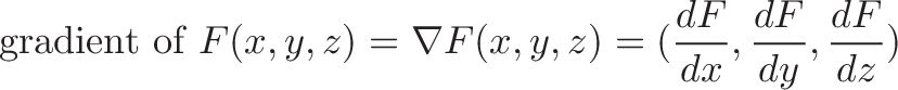
We can represent these multiple rates of change in a vector, with one component for each derivative. Thus, a function that takes 3 variables will have a gradient with 3 components:

$F(x)$ has one variable and a single derivative: $\frac{dF}{dx}$
$F(x,y,z)$ has three variables and three derivatives: $\frac{dF}{dx}, \frac{dF}{dy}, \frac{dF}{dz}$

The gradient of a multi-variable function has a component for each direction.

And just like the regular derivative, the gradient points in the direction of greatest increase (here's why: we trade motion in each direction enough to maximize the payoff).

However, now that we have multiple directions to consider ($x$, $y$ and $z$), the direction of greatest increase is no longer simply “forward” or “backward” along the $x$-axis, like it is with functions of a single variable.

If we have two variables, then our 2-component gradient can specify any direction on a plane. Likewise, with 3 variables, the gradient can specify and direction in 3D space to move to increase our function.

A Twisted Example

I’m a big fan of examples to help solidify an explanation. Suppose we have a magical oven, with coordinates written on it and a special display screen:

We can type any 3 coordinates (like “3,5,2″) and the display shows us the gradient of the temperature at that point.

The microwave also comes with a convenient clock. Unfortunately, the clock comes at a price — the temperature inside the microwave varies drastically from location to location. But this was well worth it: we really wanted that clock.

With me so far? We type in any coordinate, and the microwave spits out the gradient at that location.

Be careful not to confuse the coordinates and the gradient. The coordinates are the current location, measured on the $x,y,z$ axes. The gradient is a direction to move from our current location, such as move up, down, left or right.

Now suppose we are in need of psychiatric help and put the Pillsbury Dough Boy inside the oven because we think he would taste good. He’s made of cookie dough, right? We place him in a random location inside the oven, and our goal is to cook him as fast as possible. The gradient can help!

The gradient at any location points in the direction of greatest increase of a function. In this case, our function measures temperature. So, the gradient tells us which direction to move the doughboy to get him to a location with a higher temperature, to cook him even faster. Remember that the gradient does not give us the coordinates of where to go; it gives us the direction to move to increase our temperature.

Thus, we would start at a random point like (3,5,2) and check the gradient. In this case, the gradient there is (3,4,5). Now, we wouldn’t actually move an entire 3 units to the right, 4 units back, and 5 units up. The gradient is just a direction, so we’d follow this trajectory for a tiny bit, and then check the gradient again.

We get to a new point, pretty close to our original, which has its own gradient. This new gradient is the new best direction to follow. We’d keep repeating this process: move a bit in the gradient direction, check the gradient, and move a bit in the new gradient direction. Every time we nudged along and follow the gradient, we’d get to a warmer and warmer location.

Eventually, we’d get to the hottest part of the oven and that’s where we’d stay, about to enjoy our fresh cookies.

Don’t eat that cookie!

But before you eat those cookies, let’s make some observations about the gradient. That’s more fun, right?

First, when we reach the hottest point in the oven, what is the gradient there?

Zero. Nada. Zilch. Why? Well, once you are at the maximum location, there is no direction of greatest increase. Any direction you follow will lead to a decrease in temperature. It’s like being at the top of a mountain: any direction you move is downhill. A zero gradient tells you to stay put – you are at the max of the function, and can’t do better.

But what if there are two nearby maximums, like two mountains next to each other? You could be at the top of one mountain, but have a bigger peak next to you. In order to get to the highest point, you have to go downhill first.

Ah, now we are venturing into the not-so-pretty underbelly of the gradient. Finding the maximum in regular (single variable) functions means we find all the places where the derivative is zero: there is no direction of greatest increase. If you recall, the regular derivative will point to local minimums and maximums, and the absolute max/min must be tested from these candidate locations.

The same principle applies to the gradient, a generalization of the derivative. You must find multiple locations where the gradient is zero — you’ll have to test these points to see which one is the global maximum. Again, the top of each hill has a zero gradient — you need to compare the height at each to see which one is higher. Now that we have cleared that up, go enjoy your cookie.

Mathematics

We know the definition of the gradient: a derivative for each variable of a function. The gradient symbol is usually an upside-down delta, and called “del” (this makes a bit of sense – delta indicates change in one variable, and the gradient is the change in for all variables). Taking our group of 3 derivatives above

$\displaystyle{\text{gradient of } F(x,y,z) = \nabla F(x,y,z) = (\frac{dF}{dx},\frac{dF}{dy},\frac{dF}{dz})}$

Notice how the x-component of the gradient is the partial derivative with respect to $x$ (similar for $y$ and $z$). For a one variable function, there is no $y$-component at all, so the gradient reduces to the derivative.

Also, notice how the gradient is a function: it takes 3 coordinates as a position, and returns 3 coordinates as a direction.

$\displaystyle{F(x,y,z) = x + y^2 + z^3 }$

$\displaystyle{\nabla F(x,y,z) = (\frac{dF}{dx},\frac{dF}{dy},\frac{dF}{dz}) = (1, 2y, 3z^2)}$

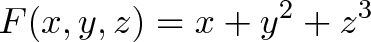
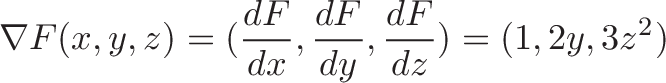
If we want to find the direction to move to increase our function the fastest, we plug in our current coordinates (such as 3,4,5) into the gradient and get:

$\displaystyle{\text{direction} = (1, 2(4), 3(5)^2) = (1, 8, 75)}$

So, this new vector (1, 8, 75) would be the direction we’d move in to increase the value of our function. In this case, our x-component doesn’t add much to the value of the function: the partial derivative is always 1.

Obvious applications of the gradient are finding the max/min of multivariable functions. Another less obvious but related application is finding the maximum of a constrained function: a function whose x and y values have to lie in a certain domain, i.e. find the maximum of all points constrained to lie along a circle. Solving this calls for my boy Lagrange, but all in due time, all in due time: enjoy the gradient for now.

The key insight is to recognize the gradient as the generalization of the derivative. The gradient points to the direction of greatest increase; keep following the gradient, and you will reach the local maximum.

Questions

Why is the gradient perpendicular to lines of equal potential?

Lines of equal potential (“equipotential”) are the points with the same energy (or value for $F(x,y,z)$). In the simplest case, a circle represents all items the same distance from the center.

The gradient represents the direction of greatest change. If it had any component along the line of equipotential, then that energy would be wasted (as it’s moving closer to a point at the same energy). When the gradient is perpendicular to the equipotential points, it is moving as far from them as possible (this article explains why the gradient is the direction of greatest increase — it’s the direction that maximizes the varying tradeoffs inside a circle).