An Intuitive Introduction To Limits

Limits, the Foundations Of Calculus, seem so artificial and weasely: “Let x approach 0, but not get there, yet we’ll act like it’s there… ” Ugh.

Here’s how I learned to enjoy them:

What is a limit? Our best prediction of a point we didn’t observe.
How do we make a prediction? Zoom into the neighboring points. If our prediction is always in-between neighboring points, no matter how much we zoom, that’s our estimate.
Why do we need limits? Math has “black hole” scenarios (dividing by zero, going to infinity), and limits give us an estimate when we can’t compute a result directly.
How do we know we’re right? We don’t. Our prediction, the limit, isn’t required to match reality. But for most natural phenomena, it sure seems to.

Limits let us ask “What if?”. If we can directly observe a function at a value (like x=0, or x growing infinitely), we don’t need a prediction. The limit wonders, “If you can see everything except a single value, what do you think is there?”.

When our prediction is consistent and improves the closer we look, we feel confident in it. And if the function behaves smoothly, like most real-world functions do, the limit is where the missing point must be.

Key Analogy: Predicting A Soccer Ball

Pretend you’re watching a soccer game. Unfortunately, the connection is choppy:

Ack! We missed what happened at 4:00. Even so, what’s your prediction for the ball’s position?

Easy. Just grab the neighboring instants (3:59 and 4:01) and predict the ball to be somewhere in-between.

And… it works! Real-world objects don’t teleport; they move through intermediate positions along their path from A to B. Our prediction is “At 4:00, the ball was between its position at 3:59 and 4:01”. Not bad.

With a slow-motion camera, we might even say “At 4:00, the ball was between its positions at 3:59.999 and 4:00.001”.

Our prediction is feeling solid. Can we articulate why?

The predictions agree at increasing zoom levels. Imagine the 3:59-4:01 range was 9.9-10.1 meters, but after zooming into 3:59.999-4:00.001, the range widened to 9-12 meters. Uh oh! Zooming should narrow our estimate, not make it worse! Not every zoom level needs to be accurate (imagine seeing the game every 5 minutes), but to feel confident, there must be some threshold where subsequent zooms only strengthen our range estimate.
The before-and-after agree. Imagine at 3:59 the ball was at 10 meters, rolling right, and at 4:01 it was at 50 meters, rolling left. What happened? We had a sudden jump (a camera change?) and now we can’t pin down the ball’s position. Which one had the ball at 4:00? This ambiguity shatters our ability to make a confident prediction.

With these requirements in place, we might say “At 4:00, the ball was at 10 meters. This estimate is confirmed by our initial zoom (3:59-4:01, which estimates 9.9 to 10.1 meters) and the following one (3:59.999-4:00.001, which estimates 9.999 to 10.001 meters)”.

Limits are a strategy for making confident predictions.

Exploring The Intuition

Let’s not bring out the math definitions just yet. What things, in the real world, do we want an accurate prediction for but can’t easily measure?

What’s the circumference of a circle?

Finding pi “experimentally” is tough: bust out a string and a ruler?

We can’t measure a shape with seemingly infinite sides, but we can wonder “Is there a predicted value for pi that is always accurate as we keep increasing the sides?”

Archimedes figured out that pi had a range of

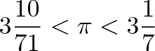
$\displaystyle{3 \frac{10}{71} < \pi < 3 \frac{1}{7} }$

using a process like this:

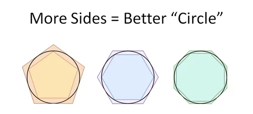
It was the precursor to calculus: he determined that pi was a number that stayed between his ever-shrinking boundaries. Nowadays, we have modern limit definitions of pi.

What does perfectly continuous growth look like?

e, one of my favorite numbers, can be defined like this:

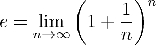
$\displaystyle{e = \lim_{n\to\infty} \left( 1 + \frac{1}{n} \right)^n}$

We can’t easily measure the result of infinitely-compounded growth. But, if we could make a prediction, is there a single rate that is ever-accurate? It seems to be around 2.71828…

Can we use simple shapes to measure complex ones?

Circles and curves are tough to measure, but rectangles are easy. If we could use an infinite number of rectangles to simulate curved area, can we get a result that withstands infinite scrutiny? (Maybe we can find the area of a circle.)

Can we find the speed at an instant?

Speed is funny: it needs a before-and-after measurement (distance traveled / time taken), but can’t we have a speed at individual instants? Hrm.

Limits help answer this conundrum: predict your speed when traveling to a neighboring instant. Then ask the “impossible question”: what’s your predicted speed when the gap to the neighboring instant is zero?

Note: The limit isn’t a magic cure-all. We can’t assume one exists, and there may not be an answer to every question. For example: Is the number of integers even or odd? The quantity is infinite, and neither the “even” nor “odd” prediction stays accurate as we count higher. No well-supported prediction exists.

For pi, e, and the foundations of calculus, smart minds did the proofs to determine that “Yes, our predicted values get more accurate the closer we look.” Now I see why limits are so important: they’re a stamp of approval on our predictions.

The Math: The Formal Definition Of A Limit

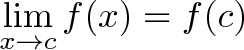
Limits are well-supported predictions. Here’s the official definition:

$\displaystyle{ \lim_{x \to c}f(x) = L }$ means for all real ε > 0 there exists a real δ > 0 such that for all x with 0 < |x − c| < δ, we have |f(x) − L| < ε

Let’s make this readable:

Math English	Human English
$\displaystyle{ \lim_{x \to c}f(x) = L \text{ means } }$	When we “strongly predict” that f(c) = L, we mean
for all real ε > 0	for any error margin we want (+/- .1 meters)
there exists a real δ > 0	there is a zoom level (+/- .1 seconds)
such that for all x with 0 < \|x − c\| < δ, we have \|f(x) − L\| < ε	where the prediction stays accurate to within the error margin

There’s a few subtleties here:

The zoom level (delta, δ) is the function input, i.e. the time in the video
The error margin (epsilon, ε) is the most the function output (the ball’s position) can differ from our prediction throughout the entire zoom level
The absolute value condition (0 < |x − c| < δ) means positive and negative offsets must work, and we’re skipping the black hole itself (when |x – c| = 0).

We can’t evaluate the black hole input, but we can say “Except for the missing point, the entire zoom level confirms the prediction $f(c) = L$.” And because $f(c) = L$ holds for any error margin we can find, we feel confident.

Could we have multiple predictions? Imagine we predicted L1 and L2 for f(c). There’s some difference between them (call it .1), therefore there’s some error margin (.01) that would reveal the more accurate one. Every function output in the range can’t be within .01 of both predictions. We either have a single, infinitely-accurate prediction, or we don’t.

Yes, we can get cute and ask for the “left hand limit” (prediction from before the event) and the “right hand limit” (prediction from after the event), but we only have a real limit when they agree.

A function is continuous when it always matches the predicted value (and discontinuous if not):

$\displaystyle{\lim_{x \to c}{f(x)} = f(c)}$

Calculus typically studies continuous functions, playing the game “We’re making predictions, but only because we know they’ll be correct.”

The Math: Showing The Limit Exists

We have the requirements for a solid prediction. Questions asking you to “Prove the limit exists” ask you to justify your estimate.

For example: Prove the limit at x=2 exists for

$\displaystyle{f(x) = \frac{(2x+1)(x-2)}{(x - 2)}}$

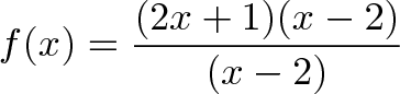
The first check: do we even need a limit? Unfortunately, we do: just plugging in “x=2” means we have a division by zero. Drats.

But intuitively, we see the same “zero” (x – 2) could be cancelled from the top and bottom. Here’s how to dance this dangerous tango:

Assume x is anywhere except 2 (It must be! We’re making a prediction from the outside.)
We can then cancel (x – 2) from the top and bottom, since it isn’t zero.
We’re left with f(x) = 2x + 1. This function can be used outside the black hole.
What does this simpler function predict? That f(2) = 2*2 + 1 = 5.

So f(2) = 5 is our prediction. But did you see the sneakiness? We pretended x wasn’t 2 [to divide out (x-2)], then plugged in 2 after that troublesome item was gone! Think of it this way: we used the simple behavior from outside the event to predict the gnarly behavior at the event.

We can prove these shenanigans give a solid prediction, and that f(2) = 5 is infinitely accurate.

For any accuracy threshold (ε), we need to find the “zoom range” (δ) where we stay within the given accuracy. For example, can we keep the estimate between +/- 1.0?

Sure. We need to find out where

$\displaystyle{|f(x) - 5| < 1.0}$

$\begin{aligned} |2x + 1 - 5| &< 1.0 \\ |2x - 4| &< 1.0 \\ |2(x - 2)| &< 1.0 \\ 2|(x - 2)| &< 1.0 \\ |x - 2| &< 0.5 \end{aligned}$

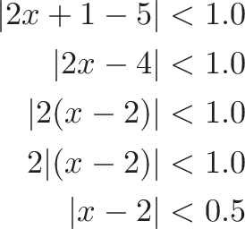
In other words, x must stay within 0.5 of 2 to maintain the initial accuracy requirement of 1.0. Indeed, when x is between 1.5 and 2.5, f(x) goes from f(1.5) = 4 to and f(2.5) = 6, staying +/- 1.0 from our predicted value of 5.

We can generalize to any error tolerance (ε) by plugging it in for 1.0 above. We get:

$\displaystyle{|x - 2| < 0.5 \cdot \epsilon}$

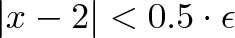
If our zoom level is “δ = 0.5 * ε”, we’ll stay within the original error. If our error is 1.0 we need to zoom to .5; if it’s 0.1, we need to zoom to 0.05.

This simple function was a convenient example. The idea is to start with the initial constraint (|f(x) – L| < ε), plug in f(x) and L, and solve for the distance away from the black-hole point (|x – c| < ?). It’s often an exercise in algebra.

Sometimes you’re asked to simply find the limit (plug in 2 and get f(2) = 5), other times you’re asked to prove a limit exists, i.e. crank through the epsilon-delta algebra.

Flipping Zero and Infinity

Infinity, when used in a limit, means “grows without stopping”. The symbol ∞ is no more a number than the sentence “grows without stopping” or “my supply of underpants is dwindling”. They are concepts, not numbers (for our level of math, Aleph me alone).

When using ∞ in a limit, we’re asking: “As x grows without stopping, can we make a prediction that remains accurate?”. If there is a limit, it means the predicted value is always confirmed, no matter how far out we look.

But, I still don’t like infinity because I can’t see it. But I can see zero. With limits, you can rewrite

$\displaystyle{\lim_{x \to \infty}}$

$\displaystyle{\lim_{\frac{1}{x} \to 0}}$

You can get sneaky and define y = 1/x, replace items in your formula, and then use

$\displaystyle{\lim_{y \to 0^+}}$

so it looks like a normal problem again! (Note from Tim in the comments: the limit is coming from the right, since x was going to positive infinity). I prefer this arrangement, because I can see the location we’re narrowing in on (we’re always running out of paper when charting the infinite version).

Why Aren’t Limits Used More Often?

Imagine a kid who figured out that “Putting a zero on the end” made a number 10x larger. Have 5? Write down “5” then “0” or 50. Have 100? Make it 1000. And so on.

He didn’t figure out why multiplication works, why this rule is justified… but, you’ve gotta admit, he sure can multiply by 10. Sure, there are some edge cases (Would 0 become “00”?), but it works pretty well.

The rules of calculus were discovered informally (by modern standards). Newton deduced that “The derivative of $x^3$ is $3x^2$” without rigorous justification. Yet engines whirl and airplanes fly based on his unofficial results.

The calculus pedagogy mistake is creating a roadblock like “You must know Limits™ before appreciating calculus”, when it’s clear the inventors of calculus didn’t. I’d prefer this progression:

Calculus asks seemingly impossible questions: When can rectangles measure a curve? Can we detect instantaneous change?
Limits give a strategy for answering “impossible” questions (“If you can make a prediction that withstands infinite scrutiny, we’ll say it’s ok.”)
They’re a great tag-team: Calculus explores, limits verify. We memorize shortcuts for the results we verified with limits ($\frac{d}{dx} x^3 = 3x^2$), just like we memorize shortcuts for the rules we verified with multiplication (adding a zero means times 10). But it’s still nice to know why the shortcuts are justified.

Limits aren’t the only tool for checking the answers to impossible questions; infinitesimals work too. The key is understanding what we’re trying to predict, then learning the rules of making predictions.

Happy math.