Chapter 10 The Theory Of Derivatives
The last lesson showed that an infinite sequence of steps could have a finite conclusion. Let’s put it into practice, and see how breaking change into infinitely small parts can point to the true amount.
10.1 Analogy: Measuring Heart Rates
Imagine you’re a doctor trying to measure a patient’s heart rate while exercising. You put a guy on a treadmill, strap on the electrodes, and get him running. The machine spits out 180 beats per minute. That must be his heart rate, right?
Nope. That’s his heart rate when observed by doctors and covered in electrodes. Wouldn’t that scenario be stressful? And what if your Nixon-era electrodes get tangled on themselves, and tug on his legs while running?
Ah. We need the electrodes to get some measurement. But, right afterwards, we need to remove the effect of the electrodes themselves. For example, if we measure 180 bpm, and knew the electrodes added 5 bpm of stress, we’d know the true heart rate was 175.
The key is making the knowingly-flawed measurement, getting a reading, then correcting it as if the instrument was never there.
10.2 Measuring the Derivative
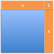
Measuring the derivative is just like putting electrodes on a function and making it run. For \( f(x) = x^2 \), we stick an electrode of \( +1 \) onto it, to see how it reacted:

The horizontal stripe is the result of our change applied along the top of the shape. The vertical stripe is our change moving along the side. And what’s the corner?
It’s part of the horizontal change interacting with the vertical one! This is an electrode getting tangled in its own wires, a measurement artifact that needs to go.
10.3 Throwing Away Artificial Results
The founders of calculus intuitively recognized which components of change were “artificial” and just threw them away. They saw that the corner piece was the result of our test measurement interacting with itself, and shouldn’t be included.
In modern times, we created official theories about how this is done:
- Limits: We let the measurement artifacts get smaller and smaller until they effectively disappear (cannot be distinguished from zero).
- Infinitesimals: Create a new type of number that lets us try infinitely-small change on a separate, tiny number system. When we bring the result back to our regular number system, the artificial elements are removed.
There are entire classes that explore these theories. The practical upshot is realizing how to take a measurement and then throwing away the parts we don’t need.
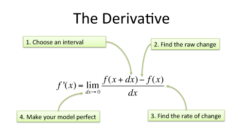
Here’s how the derivative is defined using limits:

| Step | Example |
| Start with function to study | \( f(x) = x^2 \) |
| 1. Increase the input by \( dx \), a sample change | \( f(x + dx) = (x + dx)^2 = x^2 + 2x\cdot dx + (dx)^2 \) |
| 2. Find the resulting increase in output, \( df \) | \( df = f(x + dx) - f(x) = 2x\cdot dx + (dx)^2 \) |
| 3. Find the ratio of output change to input change | \( \frac{df}{dx} = \frac{2x\cdot dx + (dx)^2}{dx} = 2x + dx \) |
| 4. Throw away any measurement artifacts | \( 2x + dx \overset{dx \ = \ 0} \Longrightarrow 2x \) |
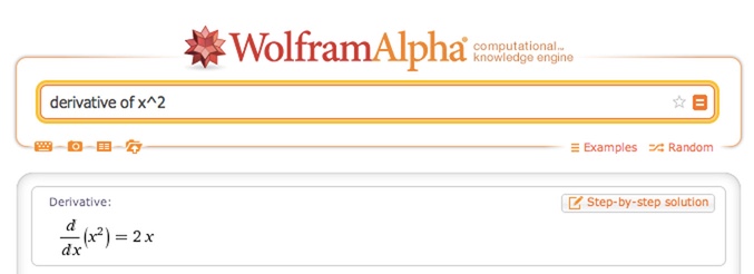
Wow! We found the official derivative for \( \frac{d}{dx} x^2 \) on our own:

Now, a few questions:
- Why do we measure \( \frac{df}{dx} \), and not the actual change \( df \)? Think of \( df \) as the entire change that happened as we took a step. For easy comparison to other functions, we typically want the “per step” change \( \frac{df}{dx} \). (This is like comparing jobs by dollars/hour instead of by salary, or cars by miles-per-gallon instead of gallons used.) Sometimes the total change is helpful to consider, and we can rewrite \( \frac{df}{dx} = 2x \) as \( df = 2x \cdot dx \).
- How can we just set \( dx \) to zero at the end? I see \( dx \) as the size of the instrument used to measure the change in a function. After we have the measurement with a real instrument (\( \frac{df}{dx} = 2x + dx \)), we figure out what the measurement would be if the instrument were perfect and did not interfere (\( \frac{df}{dx} = 2x + 0 = 2x \)).
- But isn’t the \( 2x + 1 \) pattern correct? The whole numbers (integers) are separated by an interval of 1, so assuming \( dx = 1 \) (and not letting it disappear) is accurate: \( 2x + 1 \) correctly predicts the gap of 5 between \( 2^2 \) and \( 3^2 \). However, decimals (real numbers) don’t have a fixed interval between neighbors. \( 2x \) is the ideal estimate for the rate of change between \( 2^2 \) and the infinitely-close number that follows – not 2.0001, or 2.0000000001, but whatever unnamed number comes next. Said another way, if \( dx \) doesn’t disappear, we’re saying the real numbers have a fixed interval between them, like the integers.
- If there’s no ‘+1’, when is the corner filled in? Think about the change in area, and not the specifics of the diagram. The corner overestimates how much growth happens on this step (i.e., the radar clocked us at \( 2x + 1 \) but we’re only growing by \( 2x \)). But we’re still moving and make progress.
I imagine a square that grows by bulging out its sides (\( x + x = 2x \)), then absorbing the new area to make a larger square. The new size is larger, but not quite big enough to fill in the corner exactly. It’s ok, because this process will still encompass the necessary area over time. \( 2x + 1 \) overestimates our growth because it assumes the horizontal and vertical slices interact to create the corner piece.
Practical conclusion: We can start with a knowingly-flawed measurement, \( f'(x) \sim 2x + dx \), and deduce the perfect result it points to: \( f'(x) = 2x \). The theories of exactly how we throw away \( dx \) aren’t necessary to master today. The key is realizing there are measurement artifacts – the shadow of the camera in the photo – that must be removed to accurately describe the true behavior.
(Still shaky about exactly how \( dx \) can appear and disappear? You’re in good company. This question took top mathematicians decades to resolve. Here’s a deeper discussion of how the theory works.)
Next → Lesson 11: The Fundamental Theorem Of Calculus (FTOC)