7.1 Finding the Derivative Of A Line

The derivative of a pattern, \( \frac{d}{dx}f(x) \), is the sequence of slices we get as we change an input variable (\( x \) is the natural choice here). How do we figure out the sequence of steps?

Well, I imagine going to Home Depot and pestering the clerk:

You: I’d like some lumber please. What will it run me?

Clerk: How much do you want?

You: Um… 1 foot, I think.

Clerk: That’ll be \$4. Anything else I can help you with?

You: Actually, it might be 2 feet.

Clerk: That’ll be \$8. Anything else I can help you with?

You: It might be 3 feet.

Clerk: (sigh) That’ll be \$12. Anything else I can help you with?

You: How about 4 feet?

We have a relationship (\( f(x) = 4x \)) and investigate it by changing the input a tiny bit. We see if there’s a change in output (there is!), then we change the input again, and so on.

In this case, it’s clear that an additional foot of fencing raises the cost by \$4. So we’ve just determined the derivative to be a constant 4, right?

Not so fast. Sure, we thought about the process and worked it out, but let’s be a little more organized (not every pattern is so simple). Can we describe our steps?

1. Get the current output, \( f(x) \). In our case, \( f(1) = 4 \).
2. Step forward by \( dx \) (1 foot, for example)
3. Find the new amount, \( f(x + dx) \). In our case, it’s \( f(1 + 1) = f(2) = 8 \).
4. Compute the difference: \( f(x + dx) - f(x) \), or 8 - 4 = 4

Ah! The difference between the next step and the current one is the size of our slice. For \( f(x) = 4x \) we have:

Increasing length by \( dx \) increases the cost by \( 4 \cdot dx \).

That statement is true, but a little awkward: it talks about the total change. Wouldn’t it be better to have a ratio, such as “cost per foot”?

We can extract the ratio with a few shortcuts:

• \( dx \) = change in our input
• \( df \) = resulting change in our output, \( f(x + dx) - f(x) \)
• \( \frac{df}{dx} \) = ratio of output change to input change

In our case, we have

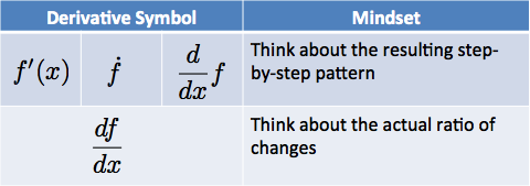
Notice how we express the derivative as \( \frac{df}{dx} \) instead of \( \frac{d}{dx}f(x) \). What gives? It turns out there’s a few different versions we can use.

Think about the various ways we express multiplication:

• Times symbol: 3 \( \times \) 4 (used in elementary school)
• Dot: 3 \( \cdot \) 4 (used in middle school)
• Implied multiplication with parentheses: \( (x + 4)(x + 3) \)
• Implied multiplication with a space: \( 2\pi r \ dr \)

The more subtle the symbol, the more we focus on the relationship between the quantities; the more visible the symbol, the more we focus on the computation.

The notation for derivatives is similar:

Some versions, like \( f'(x) \), remind us the sequence of steps is a variation of the original pattern. Notation like \( \frac{df}{dx} \) puts us into detail-oriented mode, thinking about the ratio of output change relative to the input change (“What’s the cost per additional foot?”).

Remember, the derivative is a complete description of all the steps, but it can be evaluated at a certain point to find the step there: What is the additional cost/foot when \( x = 3 \)? In our case, the answer is 4.

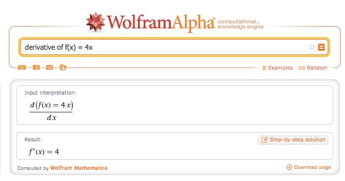
Here’s what the computer returns for this problem:

Nice! As we suspected, the pattern \( f(x) = 4x \) changes by a constant 4 as we increase \( x \).

7.2 Finding The Integral Of A Constant

Now let’s work in the other direction: given the sequence of steps, can we find the size of the original pattern?

In our fence-building scenario, it’s fairly straightforward. Solving

means answering “What pattern has an output change of 4 times the input change?”.

Well, we’ve just seen that \( f(x) = 4x \) results in \( f'(x) = 4 \). So, if we’re given \( f'(x) = 4 \), we can guess the original function must have been \( f(x) = 4x \).

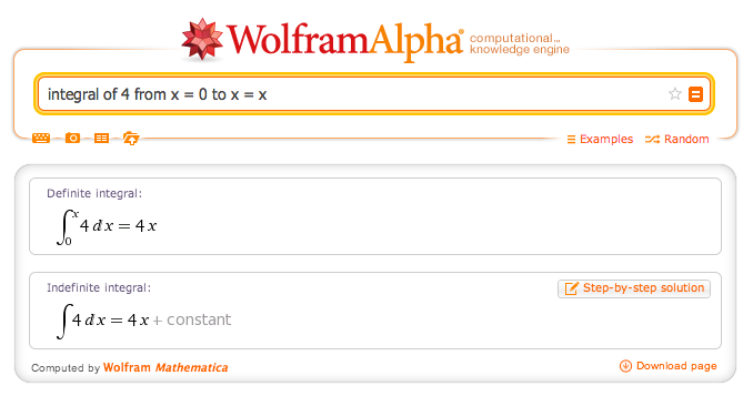
I’m pretty sure we’re right (what else could the integral of 4 be?), but let’s compare this with the computer:

Whoa – there’s two different answers (definite and indefinite). Why? Well, there’s many functions that could increase cost by \$4/foot! Here’s a few:

• Cost = \$4 per foot, or \( f(x) = 4x \)
• Cost = \$4 + \$4 per foot, or \( f(x) = 4 + 4x \)
• Cost = \$10 + \$4 per foot, or \( f(x) = 10 + 4x \)

There could be a fixed per-order fee, with the fence cost added in. All the equation \( f'(x) = 4 \) says is that each additional foot of fencing is \$4, but we don’t know the starting conditions.

• The definite integral tracks the accumulation of a set amount of slices. The range can be numbers, such as \( \int_0^{13} 4 \), which measures the slices from x=0 to x=13 (13 \( \cdot \) 4 = 52). If the range includes a variable (0 to x), then the accumulation will be an equation (\( 4x \)).
• The indefinite integral finds the actual formula that created the pattern of steps, not just the accumulation in that range. It’s written with just an integral sign: \( \int f(x) \). And as we’ve seen, the possibilities for the original function should allow for a starting offset of C.

The notation for integrals can be fast-and-loose, and it’s confusing. Are we looking for an accumulation, or the original function? Are we leaving out \( dx \)? These details are often omitted, so it’s important to feel what’s happening.

7.3 The Secret: We Can Work Backwards

The little secret of integrals is that we don’t need to solve them directly. Instead of trying to glue slices together to find out their area, we just learn to recognize the derivatives of functions we’ve already seen.

If we know the derivative of 4x is 4, then if someone asks for the integral of 4, we can respond with “4x” (plus C, of course). It’s like memorizing the squares of numbers, not the square roots. When someone asks for the square root of 121, dig through and remember that 11 \( \times \) 11 = 121.

An analogy: Imagine an antiques dealer who knows the original vase just from seeing a pile of shards.

How does he do it? Well, he takes replicas in the back room, drops them, and looks at the pattern of pieces. Then he comes to your pile and says “Oh, I think this must be a Ming Dynasty Vase from the 3rd Emperor.”

He doesn’t try to glue your pile back together – he’s just seen that exact vase break before, and your pile looks the same!

Now, there may be piles he’s never seen, that are difficult or impossible to recognize. In that case, the best he can do is to just add up the pieces (with a computer, most likely). He might determine the original vase weighed 13.78 pounds. That’s a data point, fine, but it’s not as nice as knowing what the vase was before it shattered.

This insight was never really explained to me: it’s painful to add up (possibly changing) steps directly, especially when the pattern gets complicated. So, just learn to recognize the pattern from the derivatives we’ve already seen.

7.4 Getting To Better Multiplication

Gluing together equally-sized steps looks like regular multiplication, right? You bet. If we wanted 3 steps (0 to 1, 1 to 2, 2 to 3) of size 2, we might write:

Again, this is a fancy way of saying “Accumulate 3 steps of size 2: what do you get in total?”. We are time-lapsing a sequence of equal changes.

Now, suppose someone asks you to add 2 + 2 + 2 + 2 + 2 + 2 + 2 + 2 + 2 + 2 + 2 + 2 + 2. You might say: Geez, can’t you write it more simply? You know, something like:

7.5 Creating The Abstract Rules

Have an idea how linear functions behave? Great. We can make a few abstract rules – like working out the rules of algebra for ourselves.

If we know our output is a scaled version of our input (\( f(x) = ax \)), the derivative (pattern of changes) is

and the integral (pattern of accumulation) is

That is, the ratio of each output step to each input step is a constant \( a \) (4, in our examples above). And now that we’ve broken the vase, we can work backwards: if we accumulate steps of size \( a \), they must have come from a pattern similar to \( a \cdot x \) (plus C, of course).

Notice how I wrote \( \int a \) and not \( \int a \ dx \) – I wanted to focus on \( a \), and not details like the width of the step (\( dx \)). Part of calculus is learning to expose the right amount of detail.

One last note: if our output does not react at all to our input (we’ll charge you a constant \$2 no matter how much you buy… including nothing!) then “steps” are a constant 0:

In other words, there is no difference in the before-and-after measurement. Now, a pattern may have an occasional zero slice, if it stands still for a moment. That’s fine. But if every slice were zero, it means our pattern never changes.

There are a few subtleties down the road, but let’s learn to say “Me want food” before “Verily, I hunger”.