14.1 Power Rule

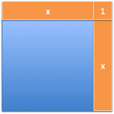
We’ve worked out that \( \frac{d}{dx}x^2 = 2x \):

We can visualize the change, and ignore the artificial corner piece. Now, how about visualizing \( x^3 \)?

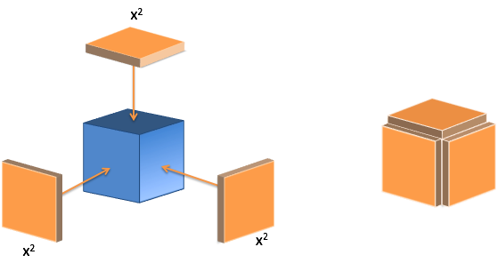
The process is similar. We can glue a plate to each side to expand the cube. The “missing gutters” represent artifacts, where our new plates would interact with each other.

I have to keep reminding myself: the gutters aren’t real! They represent growth that doesn’t happen at this step. After our growth, we “melt” the cube into its new, total area, and grow again. Counting the gutters would over-estimate the growth that happened in this step. (Now, if we’re forced to take integer-sized steps, then the gutters are needed – but with infinitely-divisible decimals, we can change smoothly.)

From the diagram, we might guess:

And that’s right! But we had to visualize the result. Abstractions like algebra let us handle scenarios we can’t visualize, like a 10-dimensional shape. Geometric shapes are a nice, visual starting point, but we need to move beyond them.

We might begin analyzing a cube with using algebra like this:

Yikes. The number of terms is getting scary, fast. What if we wanted the 10th power? Sure, there are algebra shortcuts, but let’s think about the problem holistically.

Our cube \( x^3 = x \cdot x \cdot x \) has 3 components: the sides. Call them a, b and c to keep ‘em straight. Intuitively, we know the total change has a contribution from each side:

What change does each side think it’s contributing?

• a thinks: My change (\( da \)) is combined with the other, unmoving, sides (\( b \cdot c \)) to get \( da \cdot b \cdot c \)
• b thinks: My change (\( db \)) is combined with the other sides to get \( db \cdot a \cdot c \)
• c thinks: My change (\( dc \)) is combined with the other sides to get \( dc \cdot a \cdot b \)

Each change happens separately, and there’s no “crosstalk” between \( da \), \( db \) and \( dc \) (such crosstalk leads to gutters, which we want to ignore). The total change is:

Let’s write this in terms of \( x \), the original side. Every side is identical, (\( a = b = c = x \)) and the changes are the same (\( da = db = dc = dx \)), so we get:

Converting this to a “per dx” rate we have:

Neat! Now, the brain-dead memorization strategy is to think “Pull down the exponent and decrease it by one”. That isn’t learning!

Think like this:

• \( x^3 \) has 3 identical perspectives.
• When the system changes, all 3 perspectives contribute identically. Therefore, the derivative will be \( 3 \cdot something \).
• The “something” is the change in one side (\( dx \)) multiplied by the remaining sides (\( x \cdot x \)). The changing side goes from \( x \) to \( dx \) and the exponent lowers by one.

We can reason through the rule! For example, what’s the derivative of \( x^5 \)?

Well, it’s 5 identical perspectives (\( 5 \cdot something \)). Each perspective is me changing (\( dx \)) and the 4 other guys staying the same (\( x \cdot x \cdot x \cdot x = x^4 \)). So the combined perspective is just \( 5x^4 \).

The general Power Rule:

Now we can memorize the shortcut “bring down the exponent and subtract”, just like we know that putting a 0 after a number multiplies by 10. Shortcuts are fine once you know why they work!

14.2 Integrals of Powers

Let’s try integrating a power, reverse engineering a set of changes into the original pattern.

Imagine a construction site. Day 1, they order three 1\( \times \)1 wooden planks. The next day, they order three 2\( \times \)2 wooden planks. Then three 3\( \times \)3 planks. Then three 4\( \times \)4 planks. What are they building?

My guess is a cube. They are building a shell, layer by layer, and perhaps putting grout between the gutters to glue them together.

Similarly, if we see a series of changes like \( 3x^2 \), we can visualize the plates being assembled to build a cube:

Ok – we took the previous result and worked backward. But what about the integral of plain old \( x^2 \)? Well, just imagine that incoming change is being split 3 ways:

Ah! Now we have 3 plates (each 1/3 of the original size) and we can integrate a smaller cube. Imagine the “incoming material” being split into 3 piles to build up the sides:

If we have 3 piles of size \( x^2 \), we can make a full-sized cube. Otherwise, we build a mini-cube, 1/3 as large.

The general integration rule is:

After some practice, you’ll do the division automatically. But now you know why it’s needed: we have to split the incoming “change material” among several sides. (Building a square? Share changes among 2 sides. Building a cube? Share among 3 sides. Building a 4d hypercube? Call me.)

14.3 The Quotient Rule

We’ve seen the derivative of an inverse (a “simple division”):

Remember the cake metaphor? We cut our existing portion (\( \frac{1}{x} \)) into \( x \) slices, and give one away.

Now, how can we find the derivative of \( \frac{f}{g} \)? One component in the system is trying to grow us, while the other divides us up. Which wins?

Abstraction to the rescue. When finding the derivative of \( x^3 \), we imagined it as \( x^3 = a \cdot b \cdot c \), which helped simplify the interactions. Instead of a mishmash of x’s being multiplied, it was just 3 distinct perspectives to consider.

Similarly, we can rewrite \( \frac{f}{g} \) as two perspectives:

We know \( a = f \) and \( b = \frac{1}{g} \). From this zoomed-out view, it looks like a normal, rectangular, product-rule scenario:

It’s our little secret that \( b \) is really \( \frac{1}{g} \), which behaves like a division. We just want to think about the big picture of how the rectangle changes.

Now, since \( a \) is just a rename of \( f \), we can swap in \( da = df \). But how do we swap out \( b \)? Well, we have:

Ah! This is our cake cutting. As \( g \) grows, we lose \( db = -\frac{1}{g^2} \dot dg \) from the \( b \) side. The total impact is:

This formula started with the product rule, and we plugged in their real values. Might as well put \( f \) and \( g \) back into \( (a \cdot b)' \), to get the Quotient Rule (aka the Division Rule):

Many textbooks re-arrange this relationship, like so:

And I don’t like it, no ma’am, not one bit! This version no longer resembles its ancestor, the product rule.

In practice, the Quotient Rule is a torture device designed to test your memorization skills; I rarely remember it. Just think of \( \frac{f}{g} \) as \( f \cdot \frac{1}{g} \), and use the product rule like we’ve done.

14.4 Questions

Let’s do a few warm-ups to test our skills. Can you solve these bad boys?

(You can check your answers with Wolfram Alpha, such as d/dx x⌃4.)

Again, don’t get lost in the symbols. Think “I have \( x^4 \) – what pattern of changes will I see as I make \( x \) larger?”.

Ok! How about working backwards, and doing some integrals?

Ask yourself, “What original pattern would create steps in the pattern \( 2x^2 \)?”

Trial-and-error is ok! Try a formula, test it, and adjust it. Personally, I like to move aside the 2 and just worry about the integral of \( x^2 \):

How do you know if you’re right? Take the derivative – you are the antiques dealer! I brought you a pattern of shards (\( 2x^2 \)) and you need to tell me the vase they came from. Once you have guessed a vase, break a replica in the back room and make sure you get \( 2x^2 \) back out. Then you’ll be confident in your answer (and your manager will be thrilled!).

We’re getting ready to work through the circle equations ourselves, and recreate results found by Archimedes, likely the greatest mathematician of all time.