Like making engineering students squirm? Have them explain convolution and (if you're barbarous) the convolution theorem. They'll mutter something about sliding windows as they try to escape through one.
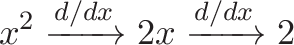
Convolution is usually introduced with its formal definition:
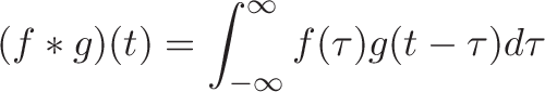
Yikes. Let's start without calculus: Convolution is fancy multiplication.
Contents
Part 1: Hospital Analogy
Imagine you manage a hospital treating patients with a single disease. You have:
- A treatment plan:
[3]Every patient gets 3 units of the cure on their first day. - A list of patients:
[1 2 3 4 5]Your patient count for the week (1 person Monday, 2 people on Tuesday, etc.).
Question: How much medicine do you use each day? Well, that's just a quick multiplication:
Plan  *  Patients       = Daily Usage
[3]   *  [1 2 3 4 5]    = [3 6 9 12 15]
Multiplying the plan by the patient list gives the usage for the upcoming days: [3 6 9 12 15]. Everyday multiplication (3 x 4) means using the plan with a single day of patients: [3] * [4] = [12].
Intuition For Convolution
Let's say the disease mutates and requires a multi-day treatment. You create a new plan: Plan: [3 2 1]
That means 3 units of the cure on the first day, 2 on the second, and 1 on the third. Ok. Given the same patient schedule [1 2 3 4 5], what's our medicine usage each day?
Uh... shoot. It's not a quick multiplication:
- On Monday, 1 patient comes in. It's her first day, so she gets 3 units.
- On Tuesday, the Monday gal gets 2 units (her second day), but two new patients arrive, who get 3 each (2 * 3 = 6). The total is 2 + (2 * 3) = 8 units.
- On Wednesday, it's trickier: The Monday gal finishes (1 unit, her last day), the Tuesday people get 2 units (2 * 2), and there are 3 new Wednesday people... argh.
The patients are overlapping and it's hard to track. How can we organize this calculation?
An idea: imagine flipping the patient list, so the first patient is on the right:
           Start of line
 5 4 3 2 1
Next, imagine we have 3 separate rooms where we apply the proper dose:
Rooms 3 2 1
On your first day, you walk into the first room and get 3 units of medicine. The next day, you walk into room #2 and get 2 units. On the last day, you walk into room #3 and get 1 unit. There's no rooms afterwards, and your treatment is done.
To calculate the total medicine usage, line up the patients and walk them through the rooms:
 Monday
 ----------------------------
 Rooms                  3 2 1
 Patients       5 4 3 2 1

 Usage                  3
On Monday (our first day), we have a single patient in the first room. She gets 3 units, for a total usage of 3. Makes sense, right?
On Tuesday, everyone takes a step forward:
 Tuesday
 ----------------------------
 Rooms                  3 2 1
 Patients ->      5 4 3 2 1

 Usage                  6 2      = 8
The first patient is now in the second room, and there's 2 new patients in the first room. We multiply each room's dose by the patient count, then combine.
Every day we just walk the list forward:
 Wednesday
 ----------------------------
 Rooms                  3 2 1
 Patients ->        5 4 3 2 1

 Usage                  9 4 1    = 14


 Thursday
 -----------------------------
 Rooms                  3 2 1
 Patients ->          5 4 3 2 1

 Usage                 12 6 2    = 20


 Friday
 -----------------------------
 Rooms                  3 2 1
 Patients ->            5 4 3 2 1

 Usage                 15 8 3    = 26
Whoa! It's intricate, but we figured it out, right? We can find the usage for any day by reversing the list, sliding it to the desired day, and combining the doses.
The total day-by-day usage looks like this (don't forget Sat and Sun, since some patients began on Friday):
Plan      *  Patient List   = Total Daily Usage

[3 2 1]   *  [1 2 3 4 5]    = [3 8 14 20 26 14 5]
              M T W T F        M T W  T  F  S  S
This calculation is the convolution of the plan and patient list. It's a fancy multiplication between a list of input numbers and a "program".
Interactive Demo
Here's a live demo. Try changing F (the plan) or G (the patient list). The convolution $c(t)$ matches our manual calculation above.
(We define functions $f(x)$ and $g(x)$ to pad each list with zero, and adjust for the list index starting at 1.)
You can do a quick convolution with Wolfram Alpha:
ListConvolve[{3, 2, 1}, {1, 2, 3, 4, 5}, {1, -1}, 0]
{3, 8, 14, 20, 26, 14, 5}
(The extra {1, -1}, 0 aligns the lists and pads with zero.)
Application: COVID Ventilator Usage
I started this article 5 years ago (intuition takes a while...), but unfortunately the analogy is relevant today.
Let's use convolution to estimate ventilator usage for incoming patients.
- Set $f(x)$ as the percent of patients needing ventilators. For example,
[.05 .03 .01]means 5% of patients need ventilators the first week, 3% the second week, and 1% the third week. - Set $g(x)$ as the weekly incoming patients, in thousands.
- The convolution $c(t) = f * g$, shows how many ventilators are needed each week (in thousands). $c(5)$ is how many ventilators are needed 5 weeks from now.
Let's try it out:
F = [.05, .03, .01]is the ventilator use percentage by weekG = [10, 20, 30, 20, 10, 10, 10], is the incoming hospitalized patients. It starts at 10k per week, rises to 30k, then decays to 10k.
With these numbers, we expect a max ventilator use of 2.2k in 2 weeks:

The convolution drops to 0 after 9 weeks because the patient list has run out. In this example, we're interested in the peak value the convolution hits, not the long-term total.
Other plans to convolve may be drug doses, vaccine appointments (one today, another a month from now), reinfections, and other complex interactions.
The hospital analogy is the mental model I wish I had when learning. Now that we've tried it with actual numbers, let's add the Math Juice and convert the analogy to calculus.
Part 2: The Calculus Definition
So, what happened in our example? We had a list of patients and a plan. If the plan were simple (single day [3]), regular multiplication would have worked. Because the plan was complex, we had to "convolve" it.
Time for some Fun Facts™:
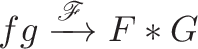
Convolution is written $f * g$, with an asterisk. Yes, an asterisk usually indicates multiplciation, but in advanced calculus class, it indicates a convolution. Regular multiplication is just implied ($fg$).
The result of a convolution is a new function that gives the total usage for any day ("What was the total usage on day $t=3$?"). We can graph the convolution over time to see the day-by-day totals.
Now the big aha: Convolution reverses one of the lists! Here's why.
Let's call our treatment plan $f(x)$. In our example, we used [3 2 1].
The list of patients (inputs) is $g(x)$. However, we need to reverse this list as we slide it, so the earliest patient (Monday) enters the hospital first (first in, first out). This means we need to use $g(-x)$, the horizontal reflection of $g(x)$. [1 2 3 4 5] becomes [5 4 3 2 1].
Now that we have the reversed list, pick a day to compute ($t = 0, 1, 2...$). To slide our patient list by this much, we use: $g(-x + t)$. That is, we reverse the list ($-x$) and jump to the correct day ($+t$).
We have our scenario:
- $f(x)$ is the plan to use
- $g(-x + t)$ is the list of inputs (flipped and slid to the right day).
To get the total usage on day $t$, we multiply each patient with the plan, and sum the results (an integral). To account for any possible length, we go from -infinity to +infinity.
Now we can describe convolution formally using calculus:
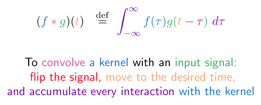
(Like colorized math? There's more.)
Phew! That's quite few symbols. Some notes:
- We use a dummy variable $\tau$ (tau) for the intermediate computation. Imagine $\tau$ as knocking on each room ($\tau={0, 1, 2, 3...}$), finding the dosage [$f(\tau)$], the number of patients [$g(t - \tau)$], multiplying them, and totaling things in the integral. Yowza. The so-called "dummy" variable $\tau$ is like
iin aforloop: it's temporary, but does the work. (By analogy, $t$ is a global variable has a fixed value during the loop: it's the day we're calculating the usage for, such ast = Day 5). - In the official definition, you'll see $g(t - \tau)$ instead of $g(- \tau+ t)$. The second version shows the flip ($-\tau$) and slide ($+t$). Writing $g(t - \tau)$ makes it seem like we're interested in the difference between the variables, which confused me.
- The treatment plan (program to run) is called the kernel: you convolve a kernel with an input.
Not too bad, right? The equation is a formal description of the analogy.
Part 3: Mathematical Properties of Convolution
We can't discover a new math operation without taking it for a spin. Let's see how it behaves.
Convolution is commutative: f * g = g * f
In our computation, we flipped the patient list and kept the plan the same. Could we have flipped the plan instead?
You bet. Imagine the patients are immobile, and stay in their rooms: [1 2 3 4 5]. To deliver the medicine, we have 3 medical carts that go to each room and deliver the dose. Each day, they slide forward one position.
  Carts ->
  1 2 3

      1 2 3 4 5
      Patients
As before, though our plan is written [3 2 1] (3 units on the first day), we flip the order of the carts to[1 2 3]. That way, a patient gets 3 units on their first day, as we expect. Checking with Wolfram Alpha, the calculation is the same.
ListConvolve[{1, 2, 3, 4, 5}, {3, 2, 1}, {1, -1}, 0]
{3, 8, 14, 20, 26, 14, 5}
Cool! It looks like convolution is commutative:
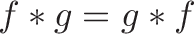
and we can decide to flip either $f$ or $g$ when calculating the integral. Surprising, right?
The integral of the convolution
When all treatments are finished, what was the total medicine usage? This is the integral of the convolution. (A few minutes ago, that phrase would have you jumping out of a window.)
But it's a simple calculation. Our plan gives each patient sum([3 2 1]) = 6 units of medicine. And we have sum([1 2 3 4 5]) = 15 patients. The total usage is just 6 x 15 = 90 units.
Wow, that was easy: the usage for the entire convolution is just the product of the subtotals!
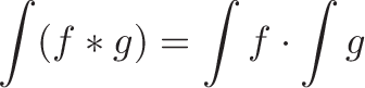
I hope this clicks intuitively. Note that this trick works for convolution, but not integrals in general. For example:
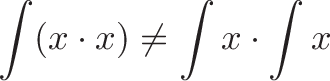
If we separate $x \cdot x$ into two integrals we get:
- $ \int (x \cdot x) = \int x^2 = \frac{1}{3} x^3 $
- $\int x \cdot \int x = \frac{1}{2}x^2 \cdot \frac{1}{2}x^2 = \frac{1}{4}x^4$
and those aren't the same. (Calculus would be much easier if we could split integrals like this.) It's strange, but $\int (f * g)$ is probably easier to solve than $\int (fg)$.
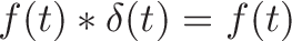
Impulse Response
What happens if we sent a single patient through the hospital? The convolution would just be that day's plan.
Plan    * Patients = Convolution
[3 2 1] * [1]      = [3 2 1]
In other words, convolving with [1] gives us the original plan.
In calculus terms, a spike of [1] (and 0 otherwise) is the Dirac Delta Function. In terms of convolutions, this function acts like the number 1 and returns the original function:
We can delay the delta function by T, which delays the resulting convolution function too. Imagine our single patient shows up a week late ($\delta(t - T)$), so our medicine usage gets delayed for a week too:

Part 4: Convolution Theorem & The Fourier Transform
The Fourier Transform (written with a fancy $\mathscr{F}$) converts a function $f(t)$ into a list of cyclical ingredients $F(s)$:
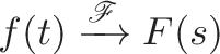
As an operator, this can be written $\mathscr{F}\lbrace f \rbrace = F$.
In our analogy, we convolved the plan and patient list with a fancy multiplication. Since the Fourier Transform gives us lists of ingredients, could we get the same result by mixing the ingredient lists?
Yep, we can: Fancy multiplication in the regular world is regular multiplication in the fancy world.
In math terms, "Convolution in the time domain is multiplication in the frequency (Fourier) domain."
Mathematically, this is written:
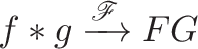
or
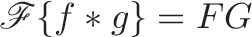
where $f(x)$ and $g(x)$ are functions to convolve, with transforms $F(s)$ and $G(s)$.
We can prove this theorem with advanced calculus, that uses theorems I don't quite understand, but let's think through the meaning.
Because $F(s)$ is the Fourier Transform of $f(t)$, we can ask for a specific frequency ($s = 2\text{Hz}$) and get the combined interaction of every data point with that frequency. Let's suppose:
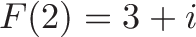
That means after every data point has been multiplied against the 2Hz cycle, the result is $3 + i$. But we could have kept each interaction separate:

Where $c_t$ is the contribution to the 2Hz frequency from datapoint $t$. Similarly, we can expand $G(s)$ into a list of interactions with the 2Hz ingredient. Let's suppose $G(2) = 7 - i$:

The Convolution Theorem is really saying:

Our convolution in the regular domain involves a lot of cross-multiplications. In the fancy frequency domain, we still have a bunch of interactions, but $F(s)$ and $G(s)$ have consolidated them. We can just multiply $F(2)G(2) = (3 + i)(7-i)$ to find the 2Hz ingredient in the convolved result.
By analogy, suppose you want to calculate:

It's a lot of work to cross-multiply every term: $(1 \cdot 5) + (1\cdot 6) + (1\cdot 7) + ...$
It's better to consolidate the groups into $(1 + 2 + 3 + 4) = 10$ and $(5 + 6 + 7 + 8) = 26$, and then multiply to get $10 \cdot 26 = 260$.
This nuance caused me a lot of confusion. It seems like $FG$ is a single multiplication, while $f * g$ involves a bunch of intermediate terms. I forgot that $F$ already did the work of merging a bunch of entries into a single one.
Now, we aren't quite done.
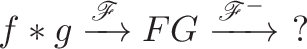
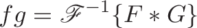
We can convert $f * g$ in the time domain into $FG$ in the frequency domain, but we probably need it back in the time domain for a usable result:
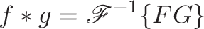
You have a riddle in English ($f * g$), you translate it to French ($FG$), get your smart French friend to work out that calculation, then convert it back to English ($\mathscr{F}^{-1}$).
And in reverse...
The convolution theorem works this way too:
Regular multiplication in the regular world is fancy multiplication in the fancy world.
Cool, eh? Instead of multiplying two functions like some cave dweller, put on your monocle, convolve the Fourier Transforms, and and convert to the time domain:
I'm not saying this is fun, just that it's possible. If your French friend has a gnarly calculation they're struggling with, it might look like arithmetic to you.
Mini proof
Remember how we said the integral of a convolution was a multiplication of the individual integrals?
Well, the Fourier Transform is just a very specific integral, right?
So (handwaving), it seems we could swap the general-purpose integral $\int$ for $\mathscr{F}$ and get

which is the convolution theorem. I need a deeper intuition for the proof, but this helps things click.
Part 5: Applications
The trick with convolution is finding a useful "program" (kernel) to apply to your input. Here's a few examples.
Moving averages
Let's say you want a moving average between neighboring items in a list. That is half of each element, added together:
This is a "multiplication program" of [0.5 0.5] convolved with our list:
ListConvolve[{1, 4, 9, 16, 25}, {0.5, 0.5}, {1, -1}, 0]
{0.5, 2.5, 6.5, 12.5, 20.5, 12.5}
We can perform a moving average with a single operation. Neat!
A 3-element moving average would be [.33 .33 .33], a weighted average could be [.5 .25 .25].
Derivatives
The derivative finds the difference between neighboring values. Here's the plan: [1 -1]
ListConvolve[{1, 2, 3, 4, 5}, {1, -1}, {1, -1}, 0]
{1, 1, 1, 1, 1, -5}                         // -5 since we ran out of entries

ListConvolve[{1, 4, 9, 16, 25}, {1, -1}, {1, -1}, 0]
{1, 3, 5, 7, 9, -25}                        // discrete derivative is 2x + 1
With a simple kernel, we can find a useful math property on a discrete list. And to get a second derivative, just apply the derivative convolution twice:
F * [1 -1] * [1 -1]
As a shortcut, we can precompute the final convolutions ([1 -1] * [1 -1] ) and get:
ListConvolve[{1, -1}, {1,-1}, {1, -1}, 0]
{1, -2, 1}
Now we have a single kernel [1, -2, 1] that gets the second derivative of a list:
ListConvolve[{1, 4, 9, 16, 25}, {1, -2, 1}, {1, -1}, 0]
{1, 2, 2, 2, 2, -34, 25}
Excluding the boundary items, we get the expected second derivative:
Blurring / unblurring images
An image blur is essentially a convolution of your image with some "blurring kernel":

The blur of our 2D image requires a 2D average:

Can we undo the blur? Yep! With our friend the Convolution Theorem, we can do:


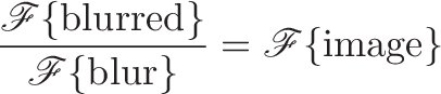
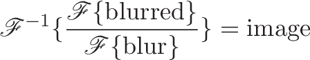
Whoa! We can recover the original image by dividing out the blur. Convolution is a simple multiplication in the frequency domain, and deconvolution is a simple division in the frequency domain.

A short while back, the concept of "deblurring by dividing Fourier Transforms" was gibberish to me. While it can be daunting mathematically, it's getting simpler conceptually.
More reading:
- Wikipedia on deconvolution, deblurring.
- Image Restoration Lecture, another one, and example for above
- Blind deconvolution is when you don't know the blur kernel (make a guess)
Algorithm Trick: Multiplication
What is a number? A list of digits:
1234 = 1000 + 200 + 30 + 4 = [1000 200 30 4]
5678 = 5000 + 600 + 70 + 8 = [5000 600 70 8]
And what is regular, grade-school multiplication? A digit-by-digit convolution! We sweep one list of digits by the other, multiplying and adding as we go:

We can perform the calculation by convolving the lists of digits (wolfram alpha):
ListConvolve[{1000, 200, 30, 4}, {8, 70, 600, 5000}, {1, -1}, 0]
{8000, 71600, 614240, 5122132, 1018280, 152400, 20000}

sum {8000, 71600, 614240, 5122132, 1018280, 152400, 20000}
7006652
Note that we pre-flip one of the lists (it gets swapped in the convolution later), and the intermediate calculations are a bit different. But, combining the subtotals gives the expected result.
Faster Convolutions
Why convolve instead of doing a regular digit-by-digit multiplication? Well, the convolution theorem lets us substitute convolution with Fourier Transforms:
The convolution ($f * g$) has complexity $O(n^2)$. We have $n$ positions to process, with $n$ intermediate multiplications at each position.
The right side involves:
- Two Fourier Transforms, which are normally $O(n^2)$. However, the Fast Fourier Transform (a divide-and-conquer approach) makes them $O(n\log(n))$.
- Pointwise multiplication of the final result of the transforms ($\sum a_n \cdot b_n$), which is $O(n)$
- An inverse transform, which is $O(n\log(n))$
And the total complexity is: $O(n\log(n)) + O(n\log(n)) + O(n) + O(n\log(n)) = O(n\log(n))$
Regular multiplication in the fancy domain is faster than a fancy multiplication in the regular domain. Our French friend is no slouch. (More)
Convolutional Neural Nets (CNN)
Machine learning is about discovering the math functions that transform input data into a desired result (a prediction, classification, etc.).
Starting with an input signal, we could convolve it with a bunch of kernels:

Given that convolution can do complex math (moving averages, blurs, derivatives...), it seems some combination of kernels should turn our input into something useful, right?
Convolutional Neural Nets (CNNs) process an input with layers of kernels, optimizing their weights (plans) to reach a goal. Imagine tweaking the treatment plan to keep medicine usage below some threshold.
CNNs are often used with image classifiers, but 1D data sets work just fine.
- Nice writeup: https://ujjwalkarn.me/2016/08/11/intuitive-explanation-convnets/
- Digit classifier demo: https://cs.stanford.edu/people/karpathy/convnetjs/demo/mnist.html
LTI System Behavior
A linear, time-invariant system means:
- Linear: Scaling and combining inputs scales and combines outputs by the same amount
- Time invariant: Outputs depend on relative time, not absolute time. You get 3 units on your first day, and it doesn't matter if it's Wednesday or Thursday.
A fancy phrase is "A LTI system is characterized by its impulse response". Translation: If we send a single patient through the hospital [1], we'll discover the treatment plan. Then we can predict the usage for any sequence of patients by convolving it with the plan.

If the system isn't LTI, we can't extrapolate based on a single person's experience. Scaling the inputs may not scale the outputs, and the actual calendar day, not relative day, may impact the result (imagine fewer rooms available on weekends).
Engineering Analogies
From David Greenspan: "Suppose you have a special laser pointer that makes a star shape on the wall. You tape together a bunch of these laser pointers in the shape of a square. The pattern on the wall now is the convolution of a star with a square."
Regular multiplication gives you a single scaled copy of an input. Convolution creates multiple overlapping copies that follow a pattern you've specified.
Real-world systems have squishy, not instantaneous, behavior: they ramp up, peak, and drop down. The convolution lets us model systems that echo, reverb and overlap.
Now it's time for the famous sliding window example. Think of a pulse of inputs (red) sliding through a system (blue), and having a combined effect (yellow): the convolution.

(Source)
Summary
Convolution has an advanced technical definition, but the basics can be understood with the right analogy.
Quick rant: I study math for fun, yet it took years to find a satisfying intuition for:
- Why is one function reversed?
- Why is convolution commutative?
- Why does the integral of the convolution = product of integrals?
- Why are the Fourier Transforms multiplied point-by-point, and not overlapped?
Why'd it take so long? Imagine learning multiplication with $f \times g = z$ instead of $3 \times 5 = 15$. Without an example I can explore in my head, I could only memorize results, not intuit them. Hopefully this analogy can save you years of struggle.
Happy math.
Other Posts In This Series
- A Visual, Intuitive Guide to Imaginary Numbers
- Intuitive Arithmetic With Complex Numbers
- Understanding Why Complex Multiplication Works
- Intuitive Guide to Angles, Degrees and Radians
- Intuitive Understanding Of Euler's Formula
- An Interactive Guide To The Fourier Transform
- Intuitive Guide to Convolution
- Intuitive Understanding of Sine Waves
- An Intuitive Guide to Linear Algebra
- A Programmer's Intuition for Matrix Multiplication
- Imaginary Multiplication vs. Imaginary Exponents
- Intuitive Guide to Hyperbolic Functions
