The average is a simple term with several meanings. The type of average to use depends on whether you’re adding, multiplying, grouping or dividing work among the items in your set.
Quick quiz: You drove to work at 30 mph, and drove back at 60 mph. What was your average speed?
Hint: It’s not 45 mph, and it doesn’t matter how far your commute is. Read on to understand the many uses of this statistical tool.

But what does it mean?
Let’s step back a bit: what is the “average” all about?
To most of us, it’s “the number in the middle” or a number that is “balanced”. I’m a fan of taking multipleviewpoints, so here’s another interpretation of the average:
The average is the value that can replace every existing item, and have the same result. If I could throw away my data and replace it with one “average” value, what would it be?
One goal of the average is to understand a data set by getting a “representative” sample. But the calculation depends on how the items in the group interact. Let’s take a look.
The Arithmetic Mean
The arithmetic mean is the most common type of average:


Let’s say you weigh 150 lbs, and are in an elevator with a 100lb kid and 350lb walrus. What’s the average weight?
The real question is “If you replaced this merry group with 3 identical people and want the same load in the elevator, what should each clone weigh?”
In this case, we’d swap in three people weighing 200 lbs each [(150 + 100 + 350)/3], and nobody would be the wiser.
Pros:
- It works well for lists that are simply combined (added) together.
- Easy to calculate: just add and divide.
- It’s intuitive — it’s the number “in the middle”, pulled up by large values and brought down by smaller ones.
Cons:
- The average can be skewed by outliers — it doesn’t deal well with wildly varying samples. The average of 100, 200 and -300 is 0, which is misleading.
The arithmetic mean works great 80% of the time; many quantities are added together. Unfortunately, there’s always those 20% of situations where the average doesn’t quite fit.
Median
The median is “the item in the middle”. But doesn’t the average (arithmetic mean) imply the same thing? What gives?
Humor me for a second: what’s the “middle” of these numbers?
- 1, 2, 3, 4, 100
Well, 3 is the middle of the list. And although the average (22) is somewhere in the “middle”, 22 doesn’t really represent the distribution. We’re more likely to get a number closer to 3 than to 22. The average has been pulled up by 100, an outlier.
The median solves this problem by taking the number in the middle of a sorted list. If there’s two middle numbers (even number of items), just take their average. Outliers like 100 only tug the median along one item in the sorted list, instead of making a drastic change: the median of 1 2 3 4 is 2.5.

Pros:
- Handles outliers well — often the most accurate representation of a group
- Splits data into two groups, each with the same number of items
Cons:
- Can be harder to calculate: you need to sort the list first
- Not as well-known; when you say “median”, people may think you mean “average”
Some jokes run along the lines of “Half of all drivers are below average. Scary, isn’t it?”. But really, in your head, you know they should be saying “half of all drivers are below median“.
Figures like housing prices and incomes are often given in terms of the median, since we want an idea of the middle of the pack. Bill Gates earning a few billion extra one year might bump up the average income, but it isn’t relevant to how a regular person’s wage changed. We aren’t interested in “adding” incomes or house prices together — we just want to find the middle one.
Again, the type of average to use depends on how the data is used.
Mode
The mode sounds strange, but it just means take a vote. And sometimes a vote, not a calculation, is the best way to get a representative sample of what people want.
Let’s say you’re throwing a party and need to pick a day (1 is Monday and 7 is Sunday). The “best” day would be the option that satisfies the most people: an average may not make sense. (“Bob likes Friday and Alice likes Sunday? Saturday it is!”).
Similarly, colors, movie preferences and much more can be measured with numbers. But again, the ideal choice may be the mode, not the average: the “average” color or “average” movie could be… unsatisfactory (Rambo meets Pride and Prejudice).

Pros:
- Works well for exclusive voting situations (this choice or that one; no compromise)
- Gives a choice that the most people wanted (whereas the average can give a choice that nobody wanted).
- Simple to understand
Cons:
- Requires more effort to compute (have to tally up the votes)
- “Winner takes all” — there’s no middle path
The term “mode” isn’t that common, but now you know what button to look for when playing around with your favorite statistics program.
Geometric Mean
The “average item” depends on how we use our existing elements. Most of the time, items are added together and the arithmetic mean works fine. But sometimes we need to do more. When dealing with investments, area and volume, we don’t add factors, we multiply them.
Let’s try an example. Which portfolio do you prefer, i.e. which has a better typical year?
- Portfolio A: +10%, -10%, +10%, -10%
- Portfolio B: +30%, -30%, +30%, -30%
They look pretty similar. Our everyday average (arithmetic mean) tells us they’re both rollercoasters, but should average out to zero profit or loss. And maybe B is better because it seems to gain more in the good years. Right?
Wrongo! Talk like that will get you burned on the stock market: investment returns are multiplied, not added! We can’t be all willy-nilly and use the arithmetic mean — we need to find the actual rate of return:
- Portfolio A:
- Return: 1.1 * .9 * 1.1 * .9 = .98 (2% loss)
- Year-over-year average: (.98)^(1/4) = 0.5% loss per year (this happens to be about 2%/4 because the numbers are small).
- Portfolio B:
- 1.3 * .7 * 1.3 * .7 = .83 (17% loss)
- Year-over-year average: (.83)^(1/4) = 4.6% loss per year.
A 2% vs 17% loss? That’s a huge difference! I’d stay away from both portfolios, but would choose A if forced. We can’t just add and divide the returns — that’s not how exponential growth works.

Some more examples:
- Inflation rates: You have inflation of 1%, 2%, and 10%. What was the average inflation during that time? (1.01 * 1.02 * 1.10)^(1/3) = 4.3%
- Coupons: You have coupons for 50%, 25% and 35% off. Assuming you can use them all, what’s the average discount? (i.e. What coupon could be used 3 times?). (.5 * .75 * .65)^(1/3) = 37.5%. Think of coupons as a “negative” return — for the store, anyway.
- Area: You have a plot of land 40 × 60 yards. What’s the “average” side — i.e., how large would the corresponding square be? (40 * 60)^(0.5) = 49 yards.
- Volume: You’ve got a shipping box 12 × 24 × 48 inches. What’s the “average” size, i.e. how large would the corresponding cube be? (12 * 24 * 48)^(1/3) = 24 inches.
I’m sure you can find many more examples: the geometric mean finds the “typical element” when items are multiplied together. You take a set of numbers, multiply them, and take the Nth root (where N is the number of items you're considering).
I had wondered for a long time why the geometric mean was useful — now we know.
Harmonic Mean
The harmonic mean is more difficult to visualize, but is still useful. (By the way, “harmonics” refer to numbers like 1/2, 1/3 — 1 over anything, really.) The harmonic mean helps us calculate average rates when several items are working together. Let’s take a look.
If I have a rate of 30 mph, it means I get some result (going 30 miles) for every input (driving 1 hour). When averaging the impact of multiple rates (X & Y), you need to think about outputs and inputs, not the raw numbers.
average rate = total output/total input

If we put both X and Y on a project, each doing the same amount of work, what is the average rate? Suppose X is 30 mph and Y is 60 mph. If we have them do similar tasks (drive a mile), the reasoning is:
- X takes 1/X time (1 mile = 1/30 hour)
- Y takes 1/Y time (1 mile = 1/60 hour)
Combining inputs and outputs we get:
- Total output: 2 miles (X and Y each contribute “1″)
- Total input: 1/X + 1/Y (each takes a different amount of time; imagine a relay race)
And the average rate, output/input, is:
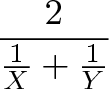
If we had 3 items in the mix (X, Y and Z) the average rate would be:
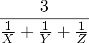
It’s nice to have this shortcut instead of doing the algebra each time — even finding the average of 5 rates isn’t so bad. With our example, we went to work at 30mph and came back at 60mph. To find the average speed, we just use the formula.
But don’t we need to know how far work is? Nope! No matter how long the route is, X and Y have the same output; that is, we go R miles at speed X, and another R miles at speed Y. The average speed is the same as going 1 mile at speed X and 1 mile at speed Y:
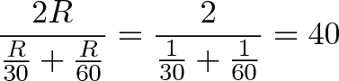
It makes sense for the average to be skewed towards the slower speed (closer to 30 than 60). After all, we spend twice as much time going 30mph than 60mph: if work is 60 miles away, it’s 2 hours there and 1 hour back.
Key idea: The harmonic mean is used when two rates contribute to the same workload. Each rate is in a relay race and contributing the same amount to the output. For example, we’re doing a round trip to work and back. Half the result (distance traveled) is from the first rate (30mph), and the other half is from the second rate (60mph).
The gotcha: Remember that the average is a single element that replaces every element. In our example, we drive 40mph on the way there (instead of 30) and drive 40 mph on the way back (instead of 60). It’s important to remember that we need to replace each “stage” with the average rate.
A few examples:
Data transmission: We’re sending data between a client and server. The client sends data at 10 gigabytes/dollar, and the server receives at 20 gigabytes/dollar. What’s the average cost? Well, we average 2 / (1/10 + 1/20) = 13.3 gigabytes/dollar for each part. That is, we could swap the client & server for two machines that cost 13.3 gb/dollar. Because data is both sent and received (each part doing “half the job”), our true rate is 13.3 / 2 = 6.65 gb/dollar.
Machine productivity: We’ve got a machine that needs to prep and finish parts. When prepping, it runs at 25 widgets/hour. When finishing, it runs at 10 widgets/hour. What’s the overall rate? Well, it averages 2 / (1/25 + 1/10) = 14.28 widgets/hour for each stage. That is, the existing times could be replaced with two phases running at 14.28 widgets/hour for the same effect. Since a part goes through both phases, the machine completes 14.28/2 = 7.14 widgets/hour.
Buying stocks. Suppose you buy \$1000 worth of stocks each month, no matter the price (dollar cost averaging). You pay \$25/share in Jan, \$30/share in Feb, and \$35/share in March. What was the average price paid? It is 3 / (1/25 + 1/30 + 1/35) = \$29.43 (since you bought more at the lower price, and less at the more expensive one). And you have \$3000 / 29.43 = 101.94 shares. The “workload” is a bit abstract — it’s turning dollars into shares. Some months use more dollars to buy a share than others, and in this case a high rate is bad.
Again, the harmonic mean helps measure rates working together on the same result.
Yikes, that was tricky
The harmonic mean is tricky: if you have separate machines running at 10 parts/hour and 20 parts/hour, then your average really is 15 parts/hour since each machine is independent and you are adding the capabilities. In that case, the arithmetic mean works just fine.
Sometimes it’s good to double-check to make sure the math works out. In the machine example, we claim to produce 7.14 widgets/hour. Ok, how long would it take to make 7.14 widgets?
- Prepping: 7.14 / 25 = .29 hours
- Finishing: 7.14 / 10 = .71 hours
And yes, .29 + .71 = 1, so the numbers work out: it does take 1 hour to make 7.14 widgets. When in doubt, try running a few examples to make sure your average rate really is what you calculated.
Conclusion
Even a simple idea like the average has many uses — there are more uses we haven’t covered (center of gravity, weighted averages, expected value). The key point is this:
- The “average item” can be seen as the item that could replace all the others
- The type of average depends on how existing items are used (Added? Multiplied? Used as rates? Used as exclusive choices?)
It surprised me how useful and varied the different types of averages were for analyzing data. Happy math.