Bayes’ theorem was the subject of a detailed article. The essay is good, but over 15,000 words long — here’s the condensed version for Bayesian newcomers like myself:
Tests are not the event. We have a cancer test, separate from the event of actually having cancer. We have a test for spam, separate from the event of actually having a spam message.
Tests are flawed. Tests detect things that don’t exist (false positive), and miss things that do exist (false negative). People often use test results without adjusting for test errors.
False positives skew results. Suppose you are searching for something really rare (1 in a million). Even with a good test, it’s likely that a positive result is really a false positive on somebody in the 999,999.
People prefer natural numbers. Saying “100 in 10,000″ rather than “1%” helps people work through the numbers with fewer errors, especially with multiple percentages (“Of those 100, 80 will test positive” rather than “80% of the 1% will test positive”).
Even science is a test. At a philosophical level, scientific experiments are “potentially flawed tests” and need to be treated accordingly. There is a test for a chemical, or a phenomenon, and there is the event of the phenomenon itself. Our tests and measuring equipment have a rate of error to be accounted for.
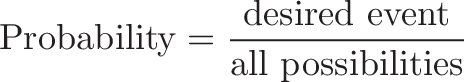
Bayes’ theorem converts the results from your test into the real probability of the event. For example, you can:
Correct for measurement errors. If you know the real probabilities and the chance of a false positive and false negative, you can correct for measurement errors.
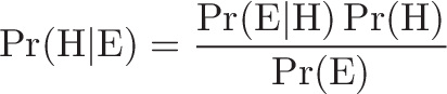
Relate the actual probability to the measured test probability. Given mammogram test results and known error rates, you can predict the actual chance of having cancer given a positive test. In technical terms, you can find Pr(H|E), the chance that a hypothesis H is true given evidence E, starting from Pr(E|H), the chance that evidence appears when the hypothesis is true.
Anatomy of a Test
The article describes a cancer testing scenario:
- 1% of women have breast cancer (and therefore 99% do not).
- 80% of mammograms detect breast cancer when it is there (and therefore 20% miss it).
- 9.6% of mammograms detect breast cancer when it’s not there (and therefore 90.4% correctly return a negative result).
Put in a table, the probabilities look like this:

How do we read it?
- 1% of people have cancer
- If you already have cancer, you are in the first column. There’s an 80% chance you will test positive. There’s a 20% chance you will test negative.
- If you don’t have cancer, you are in the second column. There’s a 9.6% chance you will test positive, and a 90.4% chance you will test negative.
How Accurate Is The Test?
Now suppose you get a positive test result. What are the chances you have cancer? 80%? 99%? 1%?
Here’s how I think about it:
- Ok, we got a positive result. It means we’re somewhere in the top row of our table. Let’s not assume anything — it could be a true positive or a false positive.
- The chances of a true positive = chance you have cancer * chance test caught it = 1% * 80% = .008
- The chances of a false positive = chance you don’t have cancer * chance test caught it anyway = 99% * 9.6% = 0.09504
The table looks like this:

And what was the question again? Oh yes: what’s the chance we really have cancer if we get a positive result. The chance of an event is the number of ways it could happen given all possible outcomes:
The chance of getting a real, positive result is .008. The chance of getting any type of positive result is the chance of a true positive plus the chance of a false positive (.008 + 0.09504 = .10304).
So, our chance of cancer is .008/.10304 = 0.0776, or about 7.8%.
Interesting — a positive mammogram only means you have a 7.8% chance of cancer, rather than 80% (the supposed accuracy of the test). It might seem strange at first but it makes sense: the test gives a false positive 9.6% of the time (quite high), so there will be many false positives in a given population. For a rare disease, most of the positive test results will be wrong.
Let’s test our intuition by drawing a conclusion from simply eyeballing the table. If you take 100 people, only 1 person will have cancer (1%), and they’re most likely going to test positive (80% chance). Of the 99 remaining people, about 10% will test positive, so we’ll get roughly 10 false positives. Considering all the positive tests, just 1 in 11 is correct, so there’s a 1/11 chance of having cancer given a positive test. The real number is 7.8% (closer to 1/13, computed above), but we found a reasonable estimate without a calculator.
Bayes’ Theorem
We can turn the process above into an equation, which is Bayes’ Theorem. It lets you take the test results and correct for the “skew” introduced by false positives. You get the real chance of having the event. Here’s the equation:
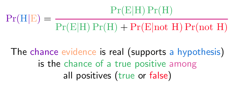
And here’s the decoder key to read it:
- Pr(H|E) = Chance of having cancer (H) given a positive test (E). This is what we want to know: How likely is it to have cancer with a positive result? In our case it was 7.8%.
- Pr(E|H) = Chance of a positive test (E) given that you had cancer (H). This is the chance of a true positive, 80% in our case.
- Pr(H) = Chance of having cancer (1%).
- Pr(not H) = Chance of not having cancer (99%).
- Pr(E|not H) = Chance of a positive test (E) given that you didn’t have cancer (not H). This is a false positive, 9.6% in our case.
Try it with any number:
It all comes down to the chance of a true positive divided by the chance of any positive. We can simplify the equation to:
Pr(E) tells us the chance of getting any positive result, whether a true positive in the cancer population (1%) or a false positive in the non-cancer population (99%). In acts like a weighting factor, adjusting the odds towards the more likely outcome.
Forgetting to account for false positives is what makes the low 7.8% chance of cancer (given a positive test) seem counter-intuitive. Thank you, normalizing constant, for setting us straight!
Intuitive Understanding: Shine The Light
The article mentions an intuitive understanding about shining a light through your real population and getting a test population. The analogy makes sense, but it takes a few thousand words to get there :).
Consider a real population. You do some tests which “shines light” through that real population and creates some test results. If the light is completely accurate, the test probabilities and real probabilities match up. Everyone who tests positive is actually “positive”. Everyone who tests negative is actually “negative”.
But this is the real world. Tests go wrong. Sometimes the people who have cancer don’t show up in the tests, and the other way around.
Bayes’ Theorem lets us look at the skewed test results and correct for errors, recreating the original population and finding the real chance of a true positive result.
Bayesian Spam Filtering
One clever application of Bayes’ Theorem is in spam filtering. We have
- Event A: The message is spam.
- Test X: The message contains certain words (X)
Plugged into a more readable formula (from Wikipedia):
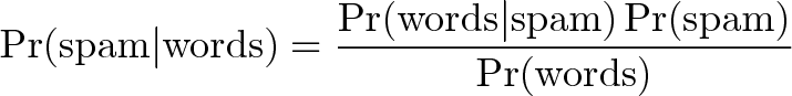
Bayesian filtering allows us to predict the chance a message is really spam given the “test results” (the presence of certain words). Clearly, words like “viagra” have a higher chance of appearing in spam messages than in normal ones.
Spam filtering based on a blacklist is flawed — it’s too restrictive and false positives are too great. But Bayesian filtering gives us a middle ground — we use probabilities. As we analyze the words in a message, we can compute the chance it is spam (rather than making a yes/no decision). If a message has a 99.9% chance of being spam, it probably is. As the filter gets trained with more and more messages, it updates the probabilities that certain words lead to spam messages. Advanced Bayesian filters can examine multiple words in a row, as another data point.
Further Reading
There’s a lot being said about Bayes:
Have fun!
