My first intuition about Bayes Theorem was “take evidence and account for false positives”. Does a lab result mean you’re sick? Well, how rare is the disease, and how often do healthy people test positive? Misleading signals must be considered.
This helped me muddle through practice problems, but I couldn’t think with Bayes. The big obstacles:
Percentages are hard to reason with. Odds compare the relative frequency of scenarios (A:B) while percentages use a part-to-whole “global scenario” [A/(A+B)]. A coin has equal odds (1:1) or a 50% chance of heads. Great. What happens when heads are 18x more likely? Well, the odds are 18:1, can you rattle off the decimal percentage? (I’ll wait…) Odds require less computation, so let’s start with them.
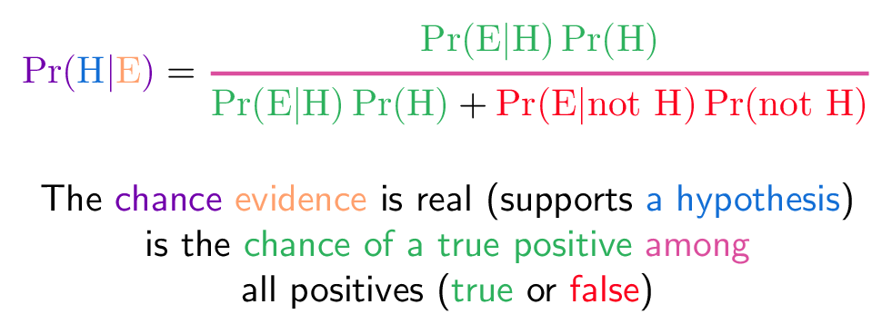
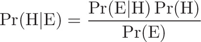
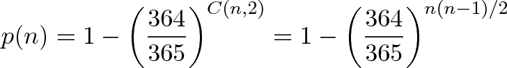
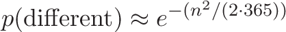
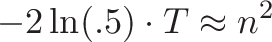
Equations miss the big picture. Here’s Bayes Theorem, as typically presented:
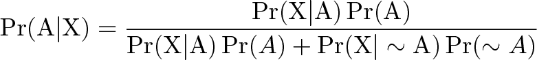
It reads right-to-left, with a mess of conditional probabilities. How about this version:
original odds * evidence adjustment = new odds
Bayes is about starting with a guess (1:3 odds for rain:sunshine), taking evidence (it’s July in the Sahara, sunshine 1000x more likely), and updating your guess (1:3000 chance of rain:sunshine). The “evidence adjustment” is how much better, or worse, we feel about our odds now that we have extra information (if it were December in Seattle, you might say rain was 1000x as likely).
Let’s start with ratios and sneak up to the complex version.
Caveman Statistician Og
Og just finished his CaveD program, and runs statistical research for his tribe:
- He saw 50 deer and 5 bears overall (50:5 odds)
- At night, he saw 10 deer and 4 bears (10:4 odds)
What can he deduce? Well,
original odds * evidence adjustment = new odds
or
evidence adjustment = new odds / original odds
At night, he realizes deer are 1/4 as likely as they were previously:
10:4 / 50:5 = 2.5 / 10 = 1/4
(Put another way, bears are 4x as likely at night)
Let’s cover ratios a bit. A:B describes how much A we get for every B (imagine miles per gallon as the ratio miles:gallon). Compare values with division: going from 25:1 to 50:1 means you doubled your efficiency (50/25 = 2). Similarly, we just discovered how our “deers per bear” amount changed.
Og happily continues his research:
- By the river, bears are 20x more likely (he saw 2 deer and 4 bears, so 2:4 / 50:5 = 1:20)
- In winter, deer are 3x as likely (30 deer and 1 bear, 30:1 / 50:5 = 3:1)
He takes a scenario, compares it to the baseline, and computes the evidence adjustment.
Caveman Clarence subscribes to Og’s journal, and wants to apply the findings to his forest (where deer:bears are 25:1). Suppose Clarence hears an animal approaching:
- His general estimate is 25:1 odds of deer:bear
- It’s at night, with bears 4x as likely => 25:4
- It’s by the river, with bears 20x as likely => 25:80
- It’s in the winter, with deer 3x more likely => 75:80
Clarence guesses “bear” with near-even odds (75:80) and tiptoes out of there.
That’s Bayes. In fancy language:
- Start with a prior probability, the general odds before evidence
- Collect evidence, and determine how much it changes the odds
- Compute the posterior probability, the odds after updating
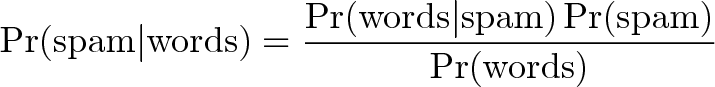
Bayesian Spam Filter
Let’s build a spam filter based on Og’s Bayesian Bear Detector.
First, grab a collection of regular and spam email. Record how often a word appears in each:
             spam      normal
hello          3         3
darling        1         5
buy            3         2
viagra         3         0
...
(“hello” appears equally, but “buy” skews toward spam)
We compute odds just like before. Let’s assume incoming email has 9:1 chance of spam, and we see “hello darling”:
- A generic message has 9:1 odds of spam:regular
- Adjust for “hello” => keep the 9:1 odds (“hello” is equally-likely in both sets)
- Adjust for “darling” => 9:5 odds (“darling” appears 5x as often in normal emails)
- Final chances => 9:5 odds of spam
We’re learning towards spam (9:5 odds). However, it’s less spammy than our starting odds (9:1), so we let it through.
Now consider a message like “buy viagra”:
- Prior belief: 9:1 chance of spam
- Adjust for “buy”: 27:2 (3:2 adjustment towards spam)
- Adjust for (“viagra”): …uh oh!
“Viagra” never appeared in a normal message. Is it a guarantee of spam?
Probably not: we should intelligently adjust for new evidence. Let’s assume there’s a regular email, somewhere, with that word, and make the “viagra” odds 3:1. Our chances become 27:2 * 3:1 = 81:2.
Now we’re geting somewhere! Our initial 9:1 guess shifts to 81:2. Now is it spam?
Well, how horrible is a false positive?
81:2 odds imply for every 81 spam messages like this, we’ll incorrectly block 2 normal emails. That ratio might be too painful. With more evidence (more words or other characteristics), we might wait for 1000:1 odds before calling a message spam.
Exploring Bayes Theorem
We can check our intuition by seeing if we naturally ask leading questions:
Is evidence truly independent? Are there links between animal behavior at night and in the winter, or words that appear together? Sure. We “naively” assume evidence is independent (and yet, in our bumbling, create effective filters anyway).
How much evidence is enough? Is seeing 2 deer & 1 bear the same 2:1 evidence adjustment as 200 deer and 100 bears?
How accurate were the starting odds in the first place? Prior beliefs change everything. (“A Bayesian is one who, vaguely expecting a horse, and catching a glimpse of a donkey, strongly believes he has seen a mule.”)
Do absolute probabilities matter? We usually need the most-likely theory (“Deer or bear?”), not the global chance of this scenario (“What’s the probability of deers at night in the winter by the river vs. bears at night in the winter by the river?”). Many Bayesian calculations ignore the global probabilities, which cancel when dividing, and essentially use an odds-centric approach.
Can our filter be tricked? A spam message might add chunks of normal text to appear innocuous and “poison” the filter. You’ve probably seen this yourself.
What evidence should we use? Let the data speak. Email might have dozens of characteristics (time of day, message headers, country of origin, HTML tags…). Give every characteristic a likelihood factor and let Bayes sort ’em out.
Thinking With Ratios and Percentages
The ratio and percentage approaches ask slightly different questions:
Ratios: Given the odds of each outcome, how does evidence adjust them?

The evidence adjustment just skews the initial odds, piece-by-piece.
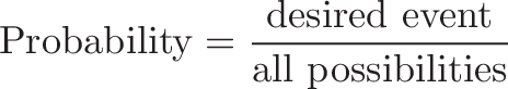
Percentages: What is the chance of an outcome after supporting evidence is found?

In the percentage case,
- “% Bears” is the overall chance of a bear appearing anywhere
- “% Bears Going to River” is how likely a bear is to trigger the “river” data point
- “% Bear at River” is the combined chance of having a bear, and it going to the river. In stats terms,
P(event and evidence) = P(event) * P(event implies evidence) = P(event) * P(evidence|event). I see conditional probabilities as “Chances that X implies Y” not the twisted “Chances of Y, given X happened”.
Let’s redo the original cancer example:
- 1% of the population has cancer
- 9.6% of healthy people test positive, 80% of people with cancer do
If you see a positive result, what’s the chance of cancer?
Ratio Approach:
- Cancer:Healthy ratio is 1:99
- Evidence adjustment: 80/100 : 9.6/100 = 80:9.6 (80% of sick people are “at the river”, and 9.6% of healthy people are).
- Final odds: 1:99 * 80:9.6 = 80:950.4 (roughly 1:12 odds of cancer, ~7.7% chance)
The intuition: the initial 1:99 odds are pretty skewed. Even with a 8.3x (80:9.6) boost from a positive test result, cancer remains unlikely.
Percentage Approach:
- Cancer chance is 1%
- Chance of true positive = 1% * 80% = .008
- Chance of false positive = 99% * 9.6% = .09504
- Chance of having cancer = .008 / (.008 + .09504) = 7.7%
When written with percentages, we start from absolute chances. There’s a global 0.8% chance of finding a sick patient with a positive result, and a global 9.504% chance of a healthy patient with a positive result. We then compute the chance these global percentages indicate something useful.
Let the approaches be complements: percentages for a bird’s-eye view, and ratios for seeing how individual odds are adjusted. We’ll save the myriad other interpretations for another day.
Happy math.